빠른 시작

---

title: 퀵스타트 description: pauli-prop Qiskit addons 패키지를 위한 퀵스타트 가이드

이 가이드에서는 pauli-prop 패키지를 사용하여 1차원 스핀 체인 위의 10 큐비트 kicked Ising 모델의 시간 동역학을 고전적으로 시뮬레이션합니다.

Pauli propagation 입력 준비하기

고려하는 해밀토니안은 다음과 같습니다.

$H = -J\sum\limits_{\langle i,j \rangle} Z_iZ_j + h\sum\limits_iX_i$

여기서 $J>0$는 최근접 스핀 $i<j$ 사이의 결합을 나타내고, $h$는 전역 횡자기장입니다. 시간 발전 연산자의 1차 Trotter 분해는 $20$개의 Trotter 단계에 걸친 양자 회로 $U$로 구현됩니다. 결합 상수 $J$는 $J=-\frac{\pi}{2}$로, $h$는 $\frac{\pi}{6}$로 고정합니다. $ZZ$ 상호작용은 Clifford 게이트($CX$, $Sdg$, $\sqrt{Y}$)로 구현합니다.

Trotter화된 시간 발전을 양자 회로로 구현하고, x축 방향의 non-Clifford 회전에는 $\frac{\pi}{6}$를 사용합니다. 이 각도가 Clifford 각도(예: $\theta=n\frac{\pi}{2}, n \in \mathbb{Z}$)에서 멀수록 Pauli propagation 방법으로 시스템을 시뮬레이션하기가 더 어려워집니다.

관측량으로는 평균 단일 사이트 자화 $\frac{1}{N} \sum_{i=1}^{N} \langle z_i \rangle$를 사용합니다. 여기서 $N$은 스핀의 개수입니다.

# Added by doQumentation — installs the packages this notebook needs if they are missing
import importlib.util

_needed = {"matplotlib": "matplotlib", "numpy": "numpy", "pauli_prop": "pauli-prop", "qiskit": "qiskit", "qiskit_aer": "qiskit-aer"}
_missing = [pip for module, pip in _needed.items()
            if importlib.util.find_spec(module) is None]
# One at a time, so a package that fails to install does not block the others
for _pip in _missing:
    %pip install -q {_pip}
if not _missing:
    print("\u2713 All required packages are installed")

import numpy as np
from qiskit import QuantumCircuit
from qiskit.quantum_info import SparsePauliOp
from qiskit.transpiler import CouplingMap

num_qubits = 10
coupling_map = CouplingMap.from_line(num_qubits, bidirectional=False)

# Num Trotter steps
num_steps = 20
theta_rx = np.pi / 6

# Average single-site magnetization
observable = (
    SparsePauliOp(
        [
            "I" * iq + "Z" + "I" * (num_qubits - iq - 1)
            for iq in range(num_qubits)
        ]
    )
    / num_qubits
)

# Create the Trotter circuit
num_qubits = 10
num_steps = 20
theta_rx = np.pi / 6
circuit = QuantumCircuit(num_qubits)
edges = CouplingMap.from_line(num_qubits, bidirectional=False).get_edges()
for _ in range(num_steps):
    circuit.rx(theta_rx, [i for i in range(num_qubits)])
    for edge in edges:
        circuit.sdg(edge)
        circuit.ry(np.pi / 2, edge[1])
        circuit.cx(edge[0], edge[1])
        circuit.ry(-np.pi / 2, edge[1])
circuit.draw("mpl", fold=-1)

Pauli propagation으로 시스템의 시간 발전 시뮬레이션하기

회로 $U$와 관측량 $O$가 준비되면 몇 단계만으로 쉽게 시스템을 시뮬레이션할 수 있습니다.

• evolve_through_cliffords를 사용해 $U$를 $U=PC$가 되도록 Clifford 부분 $C$와 non-Clifford 부분 $P$로 분리합니다

• pauli_prop.propagate_through_circuit를 사용해 $O$를 $P$를 통해 전파하여 새로운 연산자 $O^\prime$를 얻습니다

• Qiskit에 내장된 Clifford 발전 지원 기능을 사용해 $O^\prime$를 회로의 Clifford 부분을 통해 발전시킵니다

• 완전 대각 Pauli 항(모든 큐비트에서 I 또는 Z만 포함하는 Pauli 항)과 연관된 $O^\prime$의 계수를 합하여 기댓값을 $\langle0|O^\prime|0\rangle \approx \langle0|U^\dagger OU|0\rangle$로 근사합니다. 회로의 non-Clifford 부분을 통해 $O^\prime$를 전파하는 동안 항을 잘라냈기 때문에 이는 근사값이라는 점을 기억하세요.

import time

from pauli_prop import evolve_through_cliffords, propagate_through_circuit

cliff, non_cliff = evolve_through_cliffords(circuit)

max_terms_list = [10**i for i in range(8)]
approx_evs = []
durations = []
for max_terms in max_terms_list:
    st = time.perf_counter()
    evolved_obs = propagate_through_circuit(
        observable, non_cliff, max_terms=max_terms, atol=1e-12, frame="h"
    )[0]
    evolved_obs.paulis = evolved_obs.paulis.evolve(cliff, frame="h")
    durations.append(time.perf_counter() - st)
    approx_evs.append(
        float(evolved_obs.coeffs[~evolved_obs.paulis.x.any(axis=1)].sum())
    )

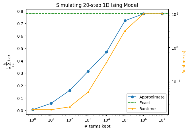
더 큰 계산을 실행할수록 기댓값 근사는 더 정확해집니다. 이 예제에서는 $4^{10}\approx10^6$ 부근에서 전체 Pauli 공간이 포화되며, 이는 마지막 두 점 사이에서 곡선이 평평해지는 것으로 나타납니다.

아래 그래프는 단조로운 수렴을 보여 주지만, Pauli propagation 시뮬레이션은 일반적으로 단조롭게 수렴하지 않습니다. 이런 종류의 그래프에서 "울퉁불퉁한" 양상을 보는 것은 드문 일이 아닙니다.

import matplotlib.pyplot as plt
from qiskit_aer import AerSimulator

sim_circ = circuit.copy()
sim_circ.save_statevector()
backend = AerSimulator(method="statevector")
psi = backend.run(sim_circ).result().data()["statevector"]
exact_ev = psi.expectation_value(observable)

ax1 = plt.gca()
ax1.plot(max_terms_list, approx_evs, marker="o", label="Approximate")
ax1.axhline(exact_ev, linestyle="--", color="green", label="Exact")
ax1.set_xscale("log")
ax1.set_xlabel("# terms kept")
ax1.set_ylabel(r"$\frac{1}{N} \sum_{i=1}^{N} \langle z_i \rangle$")

ax2 = ax1.twinx()
ax2.plot(
    max_terms_list, durations, marker=".", label="Runtime", color="orange"
)
ax2.set_ylabel("Runtime (s)", color="orange")
ax2.set_yscale("log")

handles1, labels1 = ax1.get_legend_handles_labels()
handles2, labels2 = ax2.get_legend_handles_labels()
ax1.legend(handles1 + handles2, labels1 + labels2, loc="lower right")

plt.title(f"Simulating {num_steps}-step 1D Ising Model")

Text(0.5, 1.0, 'Simulating 20-step 1D Ising Model')