CHSH 부등식
사용 시간 추정: Heron r3 프로세서에서 약 2분 (참고: 이는 추정치이며, 실제 실행 시간은 다를 수 있습니다.)
학습 성과
이 튜토리얼을 완료하면 다음 내용을 이해할 수 있습니다:
- 매개변수화된 Bell 상태 CHSH Circuit을 구성하고, CHSH 목격자를 구성하는 네 가지 기댓값을 측정하는 방법.
EstimatorV2프리미티브를 한 번 호출하여 매개변수 스윕에서 여러 관측량의 기댓값을 계산하는 방법.- 하드웨어에 제출하기 전에
AerSimulator.from_backend를 사용하여 잡음이 있는 로컬 시뮬레이터에서 양자 워크플로를 검증하는 방법. - IBM Quantum® 하드웨어에서 많은 독립적인 Bell 쌍을 병렬로 실행하여 CHSH 실험을 디바이스 전체 얽힘 벤치마크로 확장하는 방법.
사전 조건
다음 주제를 먼저 살펴보시길 권장합니다:
- 행동 속의 얽힘: Bell 상태와 CHSH 게임에 관한 강좌 레슨.
SparsePauliOp및 Qiskit 프리미티브 소개.
배경
이 튜토리얼에서는 Estimator 프리미티브를 사용하여 양자 컴퓨터에서 CHSH 부등식의 위반을 증명하는 실험을 실행합니다.
CHSH 부등식은 저자인 Clauser, Horne, Shimony, Holt의 이름을 따서 명명되었으며, 벨의 정리(1969)를 실험적으로 증명하는 데 사용됩니다. 이 정리는 국소 숨은 변수 이론이 양자역학에서 얽힘의 일부 결과를 설명할 수 없다고 주장합니다. CHSH 부등식의 위반은 양자역학이 국소 숨은 변수 이론과 양립할 수 없음을 보여주며, 이는 양자역학에 대한 우리의 이해에 있어 근본적인 실험입니다.
2022년 노벨 물리학상은 Alain Aspect, John Clauser, Anton Zeilinger에게 수여되었으며, 이는 부분적으로 양자 정보 과학에서의 선구적인 연구, 특히 얽힌 광자를 이용하여 벨 부등식의 위반을 증명한 실험에 대한 공로를 인정한 것입니다.
이 실험에서는 얽힌 쌍을 생성하고, 각 Qubit를 두 가지 다른 기저에서 측정합니다. 첫 번째 Qubit의 기저를 와 , 두 번째 Qubit의 기저를 와 로 레이블합니다. 이를 통해 CHSH 양 을 계산할 수 있습니다:
각 관측량은 또는 입니다. 분명히, 항 중 하나는 이어야 하고, 다른 하나는 이어야 합니다. 따라서 입니다. 의 평균값은 다음 부등식을 만족해야 합니다:
을 , , , 로 전개하면 다음과 같습니다:
또 다른 CHSH 양 를 정의할 수 있습니다:
이는 또 다른 부등식으로 이어집니다:
양자역학이 국소 숨은 변수 이론으로 설명될 수 있다면, 이 부등식들은 항상 성립해야 합니다. 이 튜토리얼에서 보여주듯이, 이 부등식은 양자 컴퓨터에서 위반될 수 있으므로, 양자역학은 국소 숨은 변수 이론과 양립할 수 없습니다.
벨 상태 를 준비하여 얽힌 쌍을 생성합니다. Estimator 프리미티브를 사용하면, 원시 카운트로부터 재구성하지 않고도 기댓값 , 를 직접 구할 수 있습니다. 두 번째 Qubit를 기저와 기저에서 측정합니다. 첫 번째 Qubit도 직교 기저에서 측정하지만, 회전 각도 를 에서 사이로 스윕합니다. Estimator 프리미티브는 이 매개변수 스윕을 하나의 primitive unified bloc (PUB)에서 평가합니다.
요구 사항
이 튜토리얼을 시작하기 전에 다음이 설치되어 있는지 확인하세요:
- 시각화 지원이 포함된 Qiskit SDK v2.0 이상
- Qiskit Runtime v0.40 이상 (
pip install qiskit-ibm-runtime) - Qiskit Aer v0.17 이상 (
pip install qiskit-aer)
설정
# Added by doQumentation — required packages for this notebook
!pip install -q matplotlib numpy qiskit qiskit-aer qiskit-ibm-runtime
# General
import numpy as np

# Qiskit imports
from qiskit import QuantumCircuit
from qiskit.circuit import Parameter
from qiskit.quantum_info import SparsePauliOp
from qiskit.transpiler.preset_passmanagers import generate_preset_pass_manager

# Qiskit Runtime imports
from qiskit_ibm_runtime import QiskitRuntimeService
from qiskit_ibm_runtime import EstimatorV2 as Estimator

# Qiskit Aer for local noisy simulation
from qiskit_aer import AerSimulator

# Plotting routines
import matplotlib.pyplot as plt
import matplotlib.ticker as tck
# Select an IBM Quantum backend.
service = QiskitRuntimeService()
backend = service.least_busy(
    min_num_qubits=127, operational=True, simulator=False
)
backend.name
'ibm_pittsburgh'
소규모 시뮬레이터 예제
하드웨어 작업을 제출하기 전에, 잡음이 있는 로컬 시뮬레이터에서 전체 워크플로를 검증합니다. AerSimulator.from_backend(backend)를 사용하여 선택한 Backend의 잡음 모델과 연결 맵을 상속받은 시뮬레이터를 구축합니다. 이를 통해 시뮬레이터의 응답이 하드웨어에서 예상하는 것과 질적으로 유사합니다.
1단계: 고전적 입력을 양자 문제로 매핑하기
단일 매개변수 를 가진 CHSH Circuit을 작성합니다. 이 매개변수는 첫 번째 Qubit의 측정 기저를 스윕합니다. Estimator 프리미티브는 분석을 단순화합니다: 관측량의 기댓값을 직접 반환하며, 한 번의 호출로 많은 매개변수 값에서 매개변수화된 Circuit을 평가할 수 있습니다.
theta = Parameter(r"$\theta$")

chsh_circuit = QuantumCircuit(2)
chsh_circuit.h(0)
chsh_circuit.cx(0, 1)
chsh_circuit.ry(theta, 0)
chsh_circuit.draw(output="mpl", idle_wires=False, style="iqp")

다음으로, 매개변수화된 Circuit을 평가할 에서 까지 21개의 위상 값 목록을 생성합니다 (, , , ..., , ).
number_of_phases = 21
phases = np.linspace(0, 2 * np.pi, number_of_phases)
# Phases need to be expressed as a list of lists for the Estimator PUB
individual_phases = [[ph] for ph in phases]
마지막으로 관측량을 정의합니다. 첫 번째 Qubit는 만큼 회전된 축을 따라 측정하고, 두 번째 Qubit는 및 기저에서 측정합니다. 이러한 선택에 따라 네 가지 CHSH 상관자는 파울리 연산자 , , , 로 매핑됩니다:
# <S_1> = <ZZ> - <ZX> + <XZ> + <XX>
observable1 = SparsePauliOp.from_list(
    [("ZZ", 1), ("ZX", -1), ("XZ", 1), ("XX", 1)]
)

# <S_2> = <ZZ> + <ZX> - <XZ> + <XX>
observable2 = SparsePauliOp.from_list(
    [("ZZ", 1), ("ZX", 1), ("XZ", -1), ("XX", 1)]
)
2단계: 양자 하드웨어 실행을 위한 문제 최적화
V2 프리미티브는 대상 시스템이 지원하는 명령어 및 연결성에 부합하는 Circuit과 관측량만 허용합니다 (명령어 집합 아키텍처, 즉 ISA Circuit 및 관측량). Backend로부터 AerSimulator를 구축하고, 동일한 패스 매니저가 엔드-투-엔드로 사용되도록 시뮬레이터의 대상에 대해 트랜스파일합니다.
# Build a noisy simulator from the ibm_pittsburgh backend
aer_sim = AerSimulator.from_backend(backend)

pm = generate_preset_pass_manager(target=aer_sim.target, optimization_level=3)
chsh_isa_circuit = pm.run(chsh_circuit)
chsh_isa_circuit.draw(output="mpl", idle_wires=False, style="iqp")

SparsePauliOp.apply_layout을 사용하여 트랜스파일된 Circuit의 Qubit 레이아웃에 맞게 관측량도 변환합니다.
isa_observable1 = observable1.apply_layout(layout=chsh_isa_circuit.layout)
isa_observable2 = observable2.apply_layout(layout=chsh_isa_circuit.layout)
3단계: Qiskit 프리미티브를 사용하여 실행하기
aer_sim 모드에서 EstimatorV2로 매개변수 스윕을 실행합니다. Estimator의 run() 메서드는 PUB의 이터러블을 받습니다. 각 PUB는 (circuit, observables, parameter_values, precision) 형식입니다. 두 관측량을 함께 전달하여 동일한 매개변수 스윕을 공유합니다.
# Use the AerSimulator-backed Estimator to validate the workflow locally
estimator_sim = Estimator(mode=aer_sim)

pub = (
    chsh_isa_circuit,  # ISA circuit
    [[isa_observable1], [isa_observable2]],  # ISA observables
    individual_phases,  # Parameter values
)

sim_result = estimator_sim.run(pubs=[pub]).result()
4단계: 후처리 및 원하는 고전적 형식으로 결과 반환하기
Estimator는 두 관측량의 기댓값을 반환합니다. 이를 에 대해 고전적 경계()와 Tsirelson 경계()와 함께 플롯합니다. 음영 처리된 회색 영역은 두 경계 사이의 간격을 나타냅니다. 이 영역 안에 있는 점들은 CHSH 부등식을 위반합니다.
chsh1_sim = sim_result[0].data.evs[0]
chsh2_sim = sim_result[0].data.evs[1]

def plot_chsh(phases, chsh1, chsh2, title):
    fig, ax = plt.subplots(figsize=(10, 6))

    ax.plot(
        phases / np.pi, chsh1, "o-", label=r"$\langle S_1 \rangle$", zorder=3
    )
    ax.plot(
        phases / np.pi, chsh2, "o-", label=r"$\langle S_2 \rangle$", zorder=3
    )

    # classical bound +-2
    ax.axhline(y=2, color="0.9", linestyle="--")
    ax.axhline(y=-2, color="0.9", linestyle="--")

    # quantum bound, +-2*sqrt(2)
    ax.axhline(y=np.sqrt(2) * 2, color="0.9", linestyle="-.")
    ax.axhline(y=-np.sqrt(2) * 2, color="0.9", linestyle="-.")
    ax.fill_between(phases / np.pi, 2, 2 * np.sqrt(2), color="0.6", alpha=0.7)
    ax.fill_between(
        phases / np.pi, -2, -2 * np.sqrt(2), color="0.6", alpha=0.7
    )

    ax.xaxis.set_major_formatter(tck.FormatStrFormatter("%g $\\pi$"))
    ax.xaxis.set_major_locator(tck.MultipleLocator(base=0.5))

    ax.set_xlabel(r"$\theta$")
    ax.set_ylabel("CHSH witness")
    ax.set_title(title)
    ax.legend()
    plt.show()

plot_chsh(
    phases,
    chsh1_sim,
    chsh2_sim,
    "CHSH witnesses from AerSimulator (ibm_pittsburgh noise model)",
)

시뮬레이터의 CHSH 목격자는 Backend의 잡음 모델이 적용되었음에도 불구하고, 여러 값에서 이미 고전적 경계 를 초과합니다. 피크값은 시뮬레이션된 디바이스 잡음으로 인해 Tsirelson 경계 에 약간 못 미칩니다. 워크플로를 검증했으니, 이제 실제 하드웨어로 이동합니다.
대규모 하드웨어 예제
CHSH 테스트는 본질적으로 두 Qubit 실험이므로, 하나의 Circuit을 더 크게 만드는 방식으로는 확장되지 않습니다. 대신, 많은 테스트를 병렬로 실행하는 방식으로 확장됩니다. 여기서는 Backend를 연결 맵이 허용하는 만큼의 많은 분리된 Bell 쌍으로 채우고 (연결 맵의 매칭), 모든 쌍에서 독립적인 CHSH 서브-Circuit을 하나의 작업으로 실행합니다.
이를 통해 CHSH가 디바이스 전체 얽힘 품질 벤치마크로 전환됩니다: 단일 수동 선택 쌍이 아니라, 모든 쌍이 이웃의 크로스토크 및 병렬 게이트 오류와 경쟁하는 현실적인 조건에서 칩의 상당 부분에 걸쳐 얽힘을 동시에 테스트합니다. 모든 쌍에서 동시에 부등식을 위반한다는 것은 디바이스 전체에 걸쳐 진정한 얽힘이 존재함을 인증합니다.
# -------------------------Step 1: Map classical inputs to a quantum problem-------------------------
# A CHSH test is bipartite, so we scale up by running one independent CHSH
# experiment on every disjoint Bell pair the device can host. A greedy
# matching of the coupling map gives a set of edges that share no qubits.
num_qubits = backend.num_qubits
used = set()
pairs = []
for qa, qb in backend.coupling_map.get_edges():
    if qa not in used and qb not in used:
        pairs.append((qa, qb))
        used.update((qa, qb))
num_pairs = len(pairs)
print(
    f"Tiling {backend.name} with {num_pairs} parallel Bell pairs "
    f"({2 * num_pairs} of {num_qubits} qubits)"
)

# One parameterized CHSH sub-circuit per pair, all sharing the angle theta
theta = Parameter(r"$\theta$")
chsh_circuit = QuantumCircuit(num_qubits)
for qa, qb in pairs:
    chsh_circuit.h(qa)
    chsh_circuit.cx(qa, qb)
    chsh_circuit.ry(theta, qa)

# Embed the two CHSH observables onto each pair's qubits (identity elsewhere)
obs1 = SparsePauliOp.from_list([("ZZ", 1), ("ZX", -1), ("XZ", 1), ("XX", 1)])
obs2 = SparsePauliOp.from_list([("ZZ", 1), ("ZX", 1), ("XZ", -1), ("XX", 1)])
observables = []
for qa, qb in pairs:
    observables.append([obs1.apply_layout([qa, qb], num_qubits)])
    observables.append([obs2.apply_layout([qa, qb], num_qubits)])

number_of_phases = 21
phases = np.linspace(0, 2 * np.pi, number_of_phases)
individual_phases = [[ph] for ph in phases]

# -------------------------Step 2: Optimize problem for quantum hardware execution-------------------------
pm = generate_preset_pass_manager(target=backend.target, optimization_level=3)
chsh_isa_circuit = pm.run(chsh_circuit)
isa_observables = [
    [o[0].apply_layout(chsh_isa_circuit.layout)] for o in observables
]

# -------------------------Step 3: Execute using Qiskit primitives-------------------------
estimator_hw = Estimator(mode=backend)
estimator_hw.options.environment.job_tags = ["TUT_CI"]

pub = (chsh_isa_circuit, isa_observables, individual_phases)
job = estimator_hw.run(pubs=[pub])
print(f"Job ID: {job.job_id()}")
hw_result = job.result()

# -------------------------Step 4: Post-process and return result in desired classical format-------------------------
# evs has shape (2 * num_pairs, number_of_phases); rows alternate S1, S2
evs = np.asarray(hw_result[0].data.evs)
chsh1_all = evs[0::2]
chsh2_all = evs[1::2]

# A pair "violates" CHSH if its strongest witness exceeds the classical bound
peak = np.maximum(
    np.abs(chsh1_all).max(axis=1), np.abs(chsh2_all).max(axis=1)
)
n_violate = int(np.sum(peak > 2))
print(
    f"{n_violate}/{num_pairs} Bell pairs violated the CHSH inequality "
    f"(mean peak witness {peak.mean():.2f}, classical bound 2)"
)

fig, ax = plt.subplots(figsize=(10, 6))

# Faint individual per-pair curves
for row in chsh1_all:
    ax.plot(phases / np.pi, row, color="#1f77b4", alpha=0.2, lw=1)
for row in chsh2_all:
    ax.plot(phases / np.pi, row, color="#ff7f0e", alpha=0.2, lw=1)

# Bold mean curves across all pairs
ax.plot(
    phases / np.pi,
    chsh1_all.mean(axis=0),
    color="#1f77b4",
    lw=2.5,
    label=r"$\langle S_1 \rangle$ (mean)",
)
ax.plot(
    phases / np.pi,
    chsh2_all.mean(axis=0),
    color="#ff7f0e",
    lw=2.5,
    label=r"$\langle S_2 \rangle$ (mean)",
)

# classical bound +-2 and Tsirelson bound +-2*sqrt(2)
ax.axhline(y=2, color="0.9", linestyle="--")
ax.axhline(y=-2, color="0.9", linestyle="--")
ax.axhline(y=np.sqrt(2) * 2, color="0.9", linestyle="-.")
ax.axhline(y=-np.sqrt(2) * 2, color="0.9", linestyle="-.")
ax.fill_between(phases / np.pi, 2, 2 * np.sqrt(2), color="0.6", alpha=0.7)
ax.fill_between(phases / np.pi, -2, -2 * np.sqrt(2), color="0.6", alpha=0.7)

ax.xaxis.set_major_formatter(tck.FormatStrFormatter("%g $\\pi$"))
ax.xaxis.set_major_locator(tck.MultipleLocator(base=0.5))
ax.set_xlabel(r"$\theta$")
ax.set_ylabel("CHSH witness")
ax.set_title(
    f"CHSH witnesses for {num_pairs} parallel Bell pairs on {backend.name}"
)
ax.legend()
plt.show()
Tiling ibm_pittsburgh with 64 parallel Bell pairs (128 of 156 qubits)
Job ID: d86efd5g7okc73el0rp0
63/64 Bell pairs violated the CHSH inequality (mean peak witness 2.75, classical bound 2)
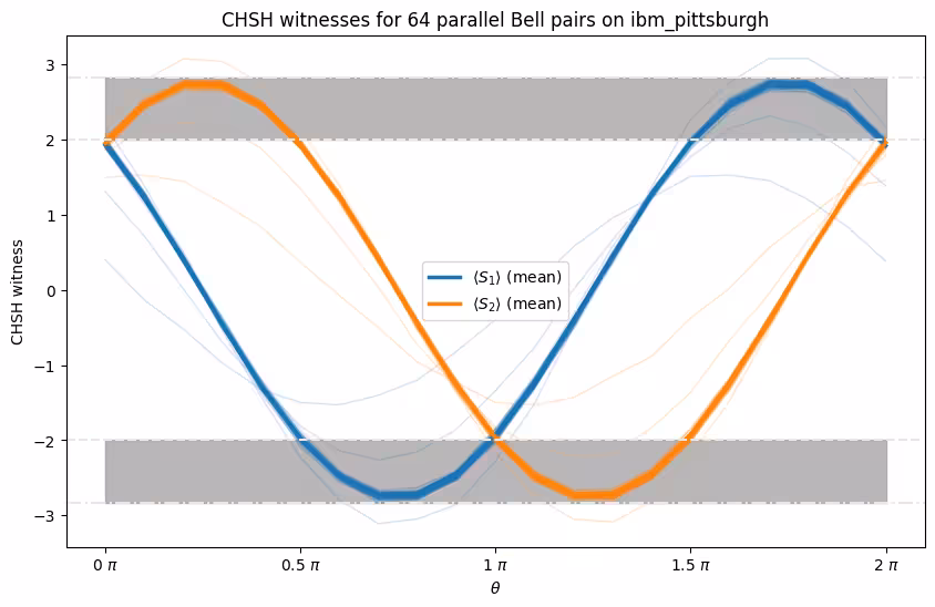
희미한 곡선은 개별 Bell 쌍을 나타내고, 굵은 곡선은 디바이스 전체의 평균입니다. 모든 쌍이 양자역학이 예측하는 동일한 사인 곡선을 추적하며, 희미한 곡선들 사이의 퍼짐은 쌍마다 잡음 변동을 반영합니다. 곡선이 회색 영역에 진입할 때마다 고전적 경계 를 넘은 것이며, 출력 요약은 본질적으로 모든 쌍이 동시에 CHSH 부등식을 위반함을 확인합니다.
피크값은 디바이스 잡음으로 인해 Tsirelson 경계 에 못 미치지만, 결론은 명확합니다: Backend는 단일 수동 선택 쌍뿐만 아니라 칩 전체에 걸쳐 동시에 진정한 얽힘을 유지합니다. 이것이 CHSH 실험이 "확장"되는 방식입니다: 더 큰 하나의 Circuit으로서가 아니라, 모든 곳에서 동시에 얽힘을 인증하는 병렬 벤치마크로서 확장됩니다.
다음 단계
이 작업이 흥미롭다고 생각하신다면, 다음 자료에도 관심을 가지실 수 있습니다:
- 행동 속의 얽힘: John Watrous의 Bell 상태와 CHSH 게임에 관한 강좌 레슨.
- Estimator 프리미티브 시작하기: PUB과 매개변수 스윕에 관한 가이드.
- Qubit 선택을 위한 실시간 벤치마킹: 디바이스 전체의 Qubit 및 얽힘 품질을 특성화하는 또 다른 방법.
SparsePauliOpAPI 참조.