화학 해밀토니안의 샘플 기반 양자 대각화

사용량 추정: Heron r2 프로세서에서 1분 미만 (참고: 이는 추정치이며 실제 실행 시간은 다를 수 있습니다.)

학습 성과

• SQD Qiskit 애드온을 사용하여 양자 처리 장치(QPU)에서 샘플링된 비트스트링으로 분자 시스템의 기저 상태 에너지를 근사하는 방법.

• ffsim을 사용하여 양자 화학 시뮬레이션을 위한 국소 유니터리 클러스터 야스트로프(LUCJ) Circuit을 구성하는 방법.

사전 요구 사항

• 양자 화학과 이차 양자화

• Sampler 프리미티브를 사용하여 양자 Circuit에서 샘플링하기

배경

이 튜토리얼에서는 SQD Qiskit 애드온을 사용하여 샘플 기반 양자 대각화(SQD) 알고리즘을 구현함으로써, 잡음 있는 양자 샘플을 후처리하여 질소 분자 $\text{N}_2$의 평형 결합 길이에서의 기저 상태를 근사하는 방법을 소개합니다. 해당 소프트웨어에 대한 자세한 내용은 관련 문서와 시작을 위한 간단한 예제에서 확인할 수 있습니다.

질소 화학은 비료를 위한 암모니아 생산을 통해 이 예제를 지속가능성과 연결합니다. 촉매가 질소를 활성화하는 방식을 이해하는 것은 에너지 소모가 적은 생산 방법에 관한 연구의 일부입니다. 고립된 질소 분자의 바닥 상태를 계산하는 것은 이러한 더 넓은 과제와 관련된 전자 구조 방법을 소개합니다.

이 튜토리얼은 양자 화학에 익숙한 사용자, 특히 분자의 기저 상태 에너지를 구하는 방법을 아는 분들에게 권장됩니다. 워크플로우에 대한 자세한 안내는 양자 대각화 알고리즘 강좌를 참조하세요.

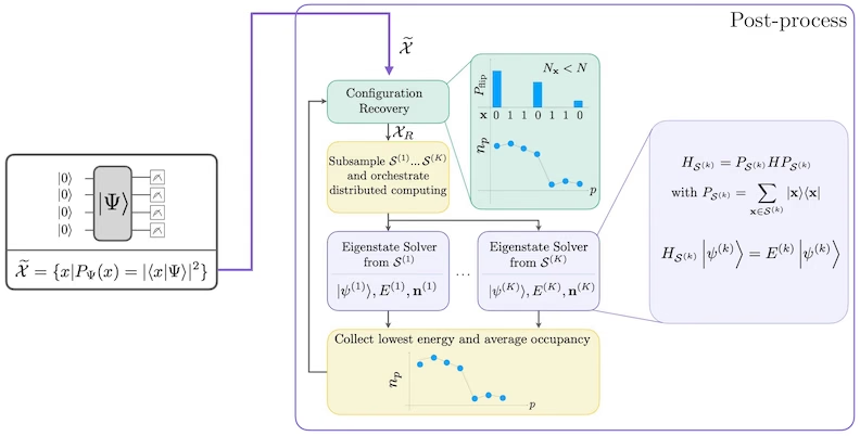
SQD는 양자 및 분산 고전 컴퓨팅을 함께 사용하여 양자 해밀토니안과 같은 양자 연산자의 고유값과 고유벡터를 찾는 기법입니다. 고전 분산 컴퓨팅은 양자 프로세서에서 얻은 샘플을 처리하고, 샘플이 형성하는 부분 공간에서 목표 해밀토니안을 투영하여 대각화하는 데 사용됩니다. SQD 기반 워크플로우는 다음 단계로 구성됩니다.

1. Circuit 앤사츠를 선택하고 양자 컴퓨터에서 기준 상태(이 경우 하트리-폭(Hartree-Fock) 상태)에 적용합니다.

2. 결과 양자 상태에서 비트스트링을 샘플링합니다.

3. 비트스트링에 대해 자기 일관적 구성 복구 절차를 실행하여 기저 상태 근사값을 구합니다.

SQD는 목표 고유상태가 희소할 때 잘 동작하는 것으로 알려져 있습니다. 즉, 파동 함수가 문제 크기에 따라 지수적으로 증가하지 않는 기저 상태(basis state) 집합 $\mathcal{S} = \{|x\rangle \}$ 위에서 지지(support)를 가질 때 효과적입니다.

양자 화학

분자 시스템의 해밀토니안은 다음과 같이 쓸 수 있습니다.

$$\hat{H} = \sum_{ \substack{pr\\\sigma} } h_{pr} \, \hat{a}^\dagger_{p\sigma} \hat{a}_{r\sigma} + \frac12 \sum_{ \substack{prqs\\\sigma\tau} } h_{prqs} \, \hat{a}^\dagger_{p\sigma} \hat{a}^\dagger_{q\tau} \hat{a}_{s\tau} \hat{a}_{r\sigma},$$

여기서 $h_{pr}$과 $h_{prqs}$는 분자 적분이라고 불리는 복소수로, 컴퓨터 프로그램을 사용하여 분자의 사양으로부터 계산됩니다. 이 튜토리얼에서는 PySCF 소프트웨어 패키지를 사용하여 적분을 계산합니다.

분자 해밀토니안의 유도 과정에 대한 자세한 내용은 양자 화학 교재(예: Szabo와 Ostlund의 Modern Quantum Chemistry)를 참고하세요. 양자 화학 문제가 양자 컴퓨터에 어떻게 매핑되는지에 대한 고수준 설명은 Qiskit Global Summer School 2024의 강의 Mapping Problems to qubits를 확인하세요.

국소 유니터리 클러스터 야스트로프(LUCJ) 앤사츠

SQD는 샘플을 추출하기 위한 양자 Circuit 앤사츠가 필요합니다. 이 튜토리얼에서는 물리적 동기와 하드웨어 친화성의 조합 덕분에 국소 유니터리 클러스터 야스트로프(LUCJ) 앤사츠를 사용합니다. 앤사츠 Circuit 구성에는 ffsim을 사용합니다.

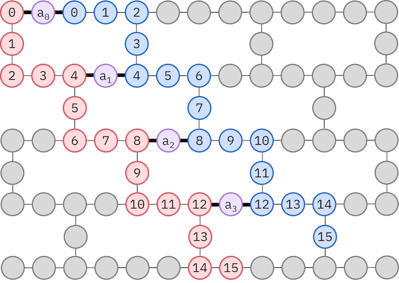
LUCJ 앤사츠는 QPU의 제한된 qubit 연결성에 적응합니다. 스핀 오비탈은 앤사츠가 SWAP Gate를 사용한 라우팅 없이 구현될 수 있도록 Qubit에 매핑됩니다. IBM® 하드웨어는 정사각 격자 또는 헤비-헥스 격자 qubit 토폴로지를 사용합니다. 헤비-헥스 격자의 경우, 아래에 나타낸 "지그재그" 패턴을 채택할 수 있습니다. 이 패턴에서 같은 스핀을 가진 오비탈은 선형 토폴로지의 Qubit에 매핑되고(빨간색과 파란색 원), 다른 스핀의 오비탈 간 연결은 4번째 공간 오비탈마다 존재하며, 보조 qubit(보라색 원)에 의해 연결이 이루어집니다.

자기 일관적 구성 복구

자기 일관적 구성 복구 절차는 잡음 있는 양자 샘플에서 가능한 한 많은 신호를 추출하도록 설계되었습니다. 분자 해밀토니안은 입자 수와 스핀 Z를 보존하므로, 이러한 대칭성을 보존하는 Circuit 앤사츠를 선택하는 것이 합리적입니다. 하트리-폭 상태에 적용하면, 잡음이 없는 경우 결과 상태는 고정된 입자 수와 스핀 Z를 가집니다. 따라서 이 상태에서 샘플링된 비트스트링의 스핀-$\alpha$ 및 스핀-$\beta$ 절반은 하트리-폭 상태와 동일한 해밍 무게를 가져야 합니다. 현재 양자 프로세서의 잡음으로 인해 일부 측정된 비트스트링은 이 특성을 위반합니다. 단순한 사후 선택 방법은 이러한 비트스트링을 버리겠지만, 이는 낭비적입니다. 왜냐하면 해당 비트스트링에도 일부 신호가 포함될 수 있기 때문입니다. 자기 일관적 복구 절차는 후처리에서 그 신호 일부를 복구하려고 시도합니다. 이 절차는 반복적이며, 기저 상태의 각 오비탈 평균 점유율 추정값을 입력으로 필요로 하고, 이 추정값은 먼저 원시 샘플에서 계산됩니다. 절차는 루프로 실행되며, 각 반복은 다음 단계로 구성됩니다.

1. 지정된 대칭성을 위반하는 각 비트스트링에 대해, 비트스트링을 현재 평균 오비탈 점유율 추정값에 더 가깝게 만들도록 설계된 확률적 절차로 비트를 뒤집어 새로운 비트스트링을 얻습니다.

2. 대칭성을 만족하는 이전 및 새 비트스트링을 모두 수집하고, 사전에 선택된 고정 크기의 부분 집합을 서브샘플링합니다.

3. 각 비트스트링 부분 집합에 대해, 해당 기저 벡터가 생성하는 부분 공간으로 해밀토니안을 투영하고(이전 섹션에서 이 기저 벡터에 대한 설명 참조), 고전 컴퓨터에서 투영된 해밀토니안의 기저 상태 추정값을 계산합니다.

4. 가장 낮은 에너지를 가진 기저 상태 추정값으로 평균 오비탈 점유율 추정값을 업데이트합니다.

SQD 워크플로우 다이어그램

SQD 워크플로우는 다음 다이어그램에 나타나 있습니다.

요구 사항

이 튜토리얼을 시작하기 전에 다음이 설치되어 있는지 확인하세요.

• Qiskit SDK v1.0 이상, 시각화 지원 포함

• Qiskit Runtime v0.22 이상 (pip install qiskit-ibm-runtime)

• SQD Qiskit 애드온 v0.12 이상 (pip install qiskit-addon-sqd)

• ffsim v0.0.75 이상 (pip install ffsim)

설정

# Added by doQumentation — installs the packages this notebook needs if they are missing
import importlib.util

_needed = {"ffsim": "ffsim", "matplotlib": "matplotlib", "numpy": "numpy", "pyscf": "pyscf", "qiskit": "qiskit", "qiskit_addon_sqd": "qiskit-addon-sqd", "qiskit_ibm_runtime": "qiskit-ibm-runtime"}
_missing = [pip for module, pip in _needed.items()
            if importlib.util.find_spec(module) is None]
# One at a time, so a package that fails to install does not block the others
for _pip in _missing:
    %pip install -q {_pip}
if not _missing:
    print("\u2713 All required packages are installed")

import math

import ffsim
import matplotlib.pyplot as plt
import numpy as np
import pyscf
import pyscf.cc
import pyscf.mcscf
from qiskit import QuantumCircuit, QuantumRegister
from qiskit.primitives import StatevectorSampler
from qiskit.providers.fake_provider import GenericBackendV2
from qiskit_ibm_runtime import QiskitRuntimeService
from qiskit_ibm_runtime import SamplerV2 as Sampler

소규모 시뮬레이터 예제

이 튜토리얼에서는 평형 결합 거리 근처의 질소 분자 기저 상태 근사값을 구합니다. 먼저 소규모 STO-6G 기저 집합을 사용하여 실험을 시뮬레이션하고 올바르게 작동하는지 확인합니다.

1단계: 고전 입력을 양자 문제로 매핑

먼저 분자와 그 특성을 지정합니다.

# Specify molecule properties
spin_sq = 0

# Build N2 molecule
mol = pyscf.gto.Mole()
mol.build(
    atom=[["N", (0, 0, -0.5)], ["N", (0, 0, 0.5)]],
    basis="sto-6g",
    symmetry="Dooh",
)

# Define active space
n_frozen = 2
active_space = range(n_frozen, mol.nao_nr())

# Get molecular integrals
scf = pyscf.scf.RHF(mol).run()
norb = len(active_space)
n_electrons = int(sum(scf.mo_occ[active_space]))
n_alpha = (n_electrons + mol.spin) // 2
n_beta = (n_electrons - mol.spin) // 2
nelec = (n_alpha, n_beta)
cas = pyscf.mcscf.CASCI(scf, norb, nelec)
mo = cas.sort_mo(active_space, base=0)
hcore, nuclear_repulsion_energy = cas.get_h1cas(mo)
eri = pyscf.ao2mo.restore(1, cas.get_h2cas(mo), norb)

# Compute exact energy using FCI
reference_energy = cas.run().e_tot

print(f"norb = {norb}")
print(f"nelec = {nelec}")

converged SCF energy = -108.464957764796
CASCI E = -108.595987350986  E(CI) = -32.4115475088426  S^2 = 0.0000000
norb = 8
nelec = (5, 5)

LUCJ 앤사츠 Circuit을 구성하기 전에, 다음 코드 셀에서 먼저 CCSD 계산을 수행합니다. 이 계산에서 얻은 $t_1$ 및 $t_2$ 진폭은 앤사츠의 매개변수를 초기화하는 데 사용됩니다.

# Get CCSD t2 amplitudes for initializing the ansatz
ccsd = pyscf.cc.CCSD(
    scf, frozen=[i for i in range(mol.nao_nr()) if i not in active_space]
).run()
t1 = ccsd.t1
t2 = ccsd.t2

E(CCSD) = -108.5933309085008  E_corr = -0.1283731437052352

이제 ffsim을 사용하여 앤사츠 Circuit을 만듭니다. 분자가 닫힌 껍질 하트리-폭 상태를 가지므로, UCJ 앤사츠의 스핀 균형 변형인 UCJOpSpinBalanced를 사용합니다. from_t_amplitudes 메서드에서 optimize=True를 설정하여 $t_2$ 진폭의 "압축된" 이중 인수분해를 활성화합니다(자세한 내용은 ffsim 문서의 The local unitary cluster Jastrow (LUCJ) ansatz 참조).

LUCJ 앤사츠는 QPU의 사용 가능한 연결성에 적응하므로, 앤사츠를 생성하기 전에 QPU Backend를 초기화해야 합니다. 여기서는 정사각 격자 커플링 맵과 LUCJ 앤사츠가 자연스럽게 분해되는 Gate 집합을 갖춘 범용 Backend를 생성합니다. 그런 다음 ffsim.qiskit.generate_lucj_pass_manager를 사용하여 "래더(ladder)" 레이아웃에 따라 주어진 Backend에 LUCJ 앤사츠를 트랜스파일하는 데 특화된 패스 매니저를 생성합니다(자세한 내용은 ffsim 문서의 설명 참조). 이 함수는 점수 휴리스틱을 사용하여 선택한 레이아웃과 관련된 오류를 최소화하는데, 이는 실제 QPU나 잡음 모델이 있는 시뮬레이터를 사용할 때 중요합니다. 패스 매니저를 반환하는 것 외에도, 하드웨어에서 구현 가능한 알파-베타 커플링 쌍도 반환합니다. 일부 쌍을 구현할 수 없는 경우 경고를 출력합니다.

import warnings

from qiskit.transpiler import CouplingMap

warnings.formatwarning = lambda msg, *args, **kwargs: f"Warning: {msg}\n"

# Set ansatz properties
n_reps = 4
pairs_aa = [(p, p + 1) for p in range(norb - 1)]

# Let generate_lucj_pass_manager determine the alpha-beta interactions
pairs_ab = None

# Initialize backend
coupling_map = CouplingMap.from_grid(norb, 2)
backend = GenericBackendV2(
    coupling_map.size(),
    coupling_map=coupling_map,
    basis_gates=["cp", "xx_plus_yy", "p", "x", "swap"],
)

# Create pass manager
pass_manager, pairs_ab = ffsim.qiskit.generate_lucj_pass_manager(
    backend=backend,
    norb=norb,
    connectivity="square",
    interaction_pairs=(pairs_aa, pairs_ab),
    optimization_level=3,
)

# Create the LUCJ ansatz operator
ucj_op = ffsim.UCJOpSpinBalanced.from_t_amplitudes(
    t2=t2,
    t1=t1,
    n_reps=n_reps,
    interaction_pairs=(pairs_aa, pairs_ab),
    # Setting optimize=True enables the "compressed" factorization
    optimize=True,
)

# create an empty quantum circuit
qubits = QuantumRegister(2 * norb, name="q")
circuit = QuantumCircuit(qubits)

# prepare Hartree-Fock state as the reference state and append it
# to the quantum circuit
circuit.append(ffsim.qiskit.PrepareHartreeFockJW(norb, nelec), qubits)

# apply the UCJ operator to the reference state
circuit.append(ffsim.qiskit.UCJOpSpinBalancedJW(ucj_op), qubits)
circuit.measure_all()

2단계: 양자 하드웨어 실행을 위한 최적화

다음으로, 대상 하드웨어에 맞게 Circuit를 최적화합니다. 일반적으로 이 단계에서는 하드웨어 Backend와 해당 Backend용 패스 매니저를 초기화합니다. 그러나 LUCJ 앤사츠가 하드웨어 연결성에 적응하므로, 이미 이전 단계에서 이 작업을 수행했습니다. 이제 패스 매니저를 Circuit에 실행하여 QPU에서 직접 실행할 수 있는 ISA Circuit으로 트랜스파일하기만 하면 됩니다.

isa_circuit = pass_manager.run(circuit)
print(f"Gate counts: {isa_circuit.count_ops()}")

Gate counts: OrderedDict({'xx_plus_yy': 254, 'cp': 88, 'p': 64, 'measure': 16, 'x': 10, 'barrier': 1})

3단계: Qiskit 프리미티브를 사용하여 실행

하드웨어 실행을 위한 Circuit 최적화가 완료되면, 대상 하드웨어에서 실행하여 바닥 상태 에너지 추정을 위한 샘플을 수집할 준비가 됩니다. Circuit가 하나뿐이므로 IBM Quantum Compute Service의 작업 실행 모드를 사용하여 Circuit를 실행합니다.

rng = np.random.default_rng(12345)
sampler = StatevectorSampler(seed=rng)
job = sampler.run([isa_circuit], shots=100_000)

primitive_result = job.result()
pub_result = primitive_result[0]

4단계: 후처리 및 원하는 고전 형식으로 결과 반환

QPU 출력의 품질을 판단하는 유용한 지표는 반환된 유효한 구성의 수입니다. 유효한 구성은 올바른 입자 수와 스핀 Z를 가지며, 이는 비트스트링의 오른쪽 절반이 스핀-업 전자 수와 같은 해밍 무게를 가지고, 왼쪽 절반이 스핀-다운 전자 수와 같은 해밍 무게를 가져야 함을 의미합니다. 다음 셀은 유효한 샘플링된 구성의 비율을 계산합니다.

def is_valid_bitstring(
    bitstring: str, norb: int, nelec: tuple[int, int]
) -> bool:
    n_alpha, n_beta = nelec
    return (
        len(bitstring) == 2 * norb
        and bitstring[norb:].count("1") == n_alpha
        and bitstring[:norb].count("1") == n_beta
    )

bit_array = pub_result.data.meas
num_valid = sum(
    is_valid_bitstring(b, norb, nelec) for b in bit_array.get_bitstrings()
)
valid_fraction = num_valid / bit_array.num_shots
print(f"Fraction of sampled configurations that are valid: {valid_fraction}")

Fraction of sampled configurations that are valid: 1.0

잡음 없는 시뮬레이터에서 Circuit를 샘플링하기 때문에 모든 비트스트링이 유효합니다. 잡음 있는 QPU에서 실행하면 비율이 1보다 작아지지만, 다음 셀에서 계산한 균일 무작위 비트스트링에서 예상되는 비율보다는 크길 바랍니다.

expected_fraction_random = (
    math.comb(norb, n_alpha) * math.comb(norb, n_beta) / 2 ** (2 * norb)
)
print(
    f"Expected fraction of valid configurations from uniformly random bitstrings: "
    f"{expected_fraction_random}"
)

Expected fraction of valid configurations from uniformly random bitstrings: 0.0478515625

이제 diagonalize_fermionic_hamiltonian 함수를 사용하여 해밀토니안의 기저 상태 에너지를 추정합니다. 이 함수는 자기 일관적 구성 복구 절차를 수행하여 잡음 있는 양자 샘플을 반복적으로 개선함으로써 에너지 추정값을 향상시킵니다. 이후 분석을 위해 중간 결과를 저장할 수 있도록 콜백 함수를 전달합니다. diagonalize_fermionic_hamiltonian의 인수 설명은 API 문서를 참조하세요.

여기서는 diagonalize_fermionic_hamiltonian의 initial_occupancies 인수를 사용하여 오비탈 점유율의 초기 추정값으로 하트리-폭 구성을 지정합니다. 이 방법은 기저 상태가 하트리-폭 구성에 상당한 지지를 가지는 시스템에 적합하지만, 다른 상황에서는 적합하지 않을 수 있습니다. 이 경우 더 고급 계산 방법을 통해 더 나은 초기 추정값을 얻을 수 있습니다. initial_occupancies를 지정하면 유효한 구성이 샘플링되지 않은 경우에도 구성 복구를 실행할 수 있습니다. 이는 잡음 있는 QPU에서 대형 Circuit를 샘플링할 때 발생할 수 있습니다. 이 인수 없이는 유효한 구성이 제공되지 않으면 구성 복구가 실패하고 오류가 발생합니다.

from functools import partial

from qiskit_addon_sqd.fermion import (
    SCIResult,
    diagonalize_fermionic_hamiltonian,
    solve_sci_batch,
)

# SQD options
energy_tol = 1e-3
occupancies_tol = 1e-3
max_iterations = 5

# Eigenstate solver options
num_batches = 3
samples_per_batch = 1000
max_dim = 50
symmetrize_spin = True
carryover_threshold = 1e-4
max_cycle = 200

# Use the Hartree-Fock configuration as an initial guess for the orbital occupancies
initial_occupancies = (
    np.array([1] * n_alpha + [0] * (norb - n_alpha)),
    np.array([1] * n_beta + [0] * (norb - n_beta)),
)

# Pass options to the built-in eigensolver. If you just want to use the defaults,
# you can omit this step, in which case you would not specify the sci_solver argument
# in the call to diagonalize_fermionic_hamiltonian below.
sci_solver = partial(solve_sci_batch, spin_sq=0.0, max_cycle=max_cycle)

# List to capture intermediate results
result_history = []

def callback(results: list[SCIResult]):
    result_history.append(results)
    iteration = len(result_history)
    print(f"Iteration {iteration}")
    for i, result in enumerate(results):
        print(f"\tSubsample {i}")
        print(f"\t\tEnergy: {result.energy + nuclear_repulsion_energy}")
        print(
            f"\t\tSubspace dimension: {np.prod(result.sci_state.amplitudes.shape)}"
        )

result = diagonalize_fermionic_hamiltonian(
    hcore,
    eri,
    bit_array,
    samples_per_batch=samples_per_batch,
    norb=norb,
    nelec=nelec,
    num_batches=num_batches,
    energy_tol=energy_tol,
    occupancies_tol=occupancies_tol,
    max_iterations=max_iterations,
    sci_solver=sci_solver,
    symmetrize_spin=symmetrize_spin,
    max_dim=max_dim,
    initial_occupancies=initial_occupancies,
    carryover_threshold=carryover_threshold,
    callback=callback,
    seed=rng,
)

final_energy = result.energy + nuclear_repulsion_energy
energy_error = final_energy - reference_energy
print(f"Final energy: {final_energy}")
print(f"Final energy error: {energy_error}")

Iteration 1
	Subsample 0
		Energy: -108.59589540253083
		Subspace dimension: 2500
	Subsample 1
		Energy: -108.59589540253083
		Subspace dimension: 2500
	Subsample 2
		Energy: -108.59589540253083
		Subspace dimension: 2500
Iteration 2
	Subsample 0
		Energy: -108.59589540253083
		Subspace dimension: 2500
	Subsample 1
		Energy: -108.59589540253083
		Subspace dimension: 2500
	Subsample 2
		Energy: -108.59589540253083
		Subspace dimension: 2500
Final energy: -108.59589540253083
Final energy error: 9.19484552071026e-05

결과 시각화

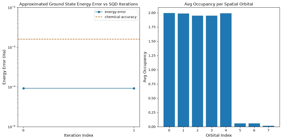
첫 번째 플롯은 이 시뮬레이션에서 첫 번째 반복 후 이미 정확한 답의 1 mH 이내에 있음을 보여줍니다 (화학적 정확도는 일반적으로 1 kcal/mol $\approx$ 1.6 mH로 허용됩니다). 그러나 이것은 소규모 시스템이며 샘플이 잡음 없이 생성되었기 때문에 구성 복구가 필요하지 않습니다. 잡음 있는 QPU에서 실행되는 더 큰 시스템의 경우, 여러 번의 구성 복구 반복이 필요할 수 있으며 최종 정확도가 더 낮을 수 있습니다. 일반적으로 구성 복구 반복 횟수를 늘리거나 배치당 샘플 수를 늘리면 에너지를 개선할 수 있습니다.

두 번째 플롯은 마지막 반복 후 각 공간 오비탈의 평균 점유율을 보여줍니다. 얻은 해에서 스핀-업 전자와 스핀-다운 전자 모두 처음 다섯 개의 오비탈을 높은 확률로 점유하고 있음을 알 수 있습니다.

# Data for energies plot
x1 = range(len(result_history))
min_e = [
    min(result, key=lambda res: res.energy).energy + nuclear_repulsion_energy
    for result in result_history
]
e_diff = [abs(e - reference_energy) for e in min_e]

# Chemical accuracy (+/- 1.6 milli-Hartree)
chem_accuracy = 0.0016

# Data for avg spatial orbital occupancy
y2 = np.sum(result.orbital_occupancies, axis=0)
x2 = range(len(y2))

fig, axs = plt.subplots(1, 2, figsize=(12, 6))

# Plot energies
axs[0].plot(x1, e_diff, label="energy error", marker="o")
axs[0].set_xticks(x1)
axs[0].set_xticklabels(x1)
axs[0].set_yscale("log")
axs[0].set_ylim(1e-5, 1e-2)
axs[0].axhline(
    y=chem_accuracy,
    color="#BF5700",
    linestyle="--",
    label="chemical accuracy",
)
axs[0].set_title("Approximated Ground State Energy Error vs SQD Iterations")
axs[0].set_xlabel("Iteration Index", fontdict={"fontsize": 12})
axs[0].set_ylabel("Energy Error (Ha)", fontdict={"fontsize": 12})
axs[0].legend()

# Plot orbital occupancy
axs[1].bar(x2, y2, width=0.8)
axs[1].set_xticks(x2)
axs[1].set_xticklabels(x2)
axs[1].set_title("Avg Occupancy per Spatial Orbital")
axs[1].set_xlabel("Orbital Index", fontdict={"fontsize": 12})
axs[1].set_ylabel("Avg Occupancy", fontdict={"fontsize": 12})

plt.tight_layout()
plt.show()

대규모 하드웨어 예제

이제 실제 양자 하드웨어에서 더 큰 예제를 실행합니다. 여기서는 cc-pVDZ 기저 집합으로부터 질소 분자의 활성 공간을 도출합니다. 또한 다음과 같은 변경을 적용합니다:

• 게이트 오류로 인한 잡음을 줄이기 위해 n_reps를 1로 낮춥니다
• Backend 프로세서 패밀리(Heron은 헤비-헥스, Nighthawk는 정사각 격자)에 따라 앤사츠 연결성을 설정합니다
• 더 큰 부분공간 차원을 허용하기 위해 max_dim을 1000으로 늘립니다.

1-4단계

여기서는 모든 단계를 더 큰 규모의 단일 워크플로우로 통합하여 실제 양자 하드웨어에서 실행합니다.

# ------------------------------ Step 1 ------------------------------
# Build N2 molecule
mol = pyscf.gto.Mole()
mol.build(
    atom=[["N", (0, 0, -0.5)], ["N", (0, 0, 0.5)]],
    basis="cc-pvdz",
    symmetry="Dooh",
)

# Define active space
n_frozen = 2
active_space = range(n_frozen, mol.nao_nr())

# Get molecular integrals
scf = pyscf.scf.RHF(mol).run()
norb = len(active_space)
n_electrons = int(sum(scf.mo_occ[active_space]))
n_alpha = (n_electrons + mol.spin) // 2
n_beta = (n_electrons - mol.spin) // 2
nelec = (n_alpha, n_beta)
cas = pyscf.mcscf.CASCI(scf, norb, nelec)
mo = cas.sort_mo(active_space, base=0)
hcore, nuclear_repulsion_energy = cas.get_h1cas(mo)
eri = pyscf.ao2mo.restore(1, cas.get_h2cas(mo), norb)

# Store reference energy from SCI calculation performed separately
reference_energy = -109.22802921665716

print(f"norb = {norb}")
print(f"nelec = {nelec}")

# Get CCSD t2 amplitudes for initializing the ansatz
ccsd = pyscf.cc.CCSD(
    scf, frozen=[i for i in range(mol.nao_nr()) if i not in active_space]
).run()
t1 = ccsd.t1
t2 = ccsd.t2

# Set ansatz properties
n_reps = 1
pairs_aa = [(p, p + 1) for p in range(norb - 1)]

# Let generate_lucj_pass_manager determine the alpha-beta interactions
pairs_ab = None

# Initialize backend
service = QiskitRuntimeService()
backend = service.least_busy(operational=True, simulator=False)
print(f"Using backend {backend.name}")

# Create pass manager
connectivity_map = {"Heron": "heavy-hex", "Nighthawk": "square"}
pass_manager, pairs_ab = ffsim.qiskit.generate_lucj_pass_manager(
    backend=backend,
    norb=norb,
    connectivity=connectivity_map[
        backend.configuration().processor_type["family"]
    ],
    interaction_pairs=(pairs_aa, pairs_ab),
    optimization_level=3,
)

# Create the LUCJ ansatz operator
ucj_op = ffsim.UCJOpSpinBalanced.from_t_amplitudes(
    t2=t2,
    t1=t1,
    n_reps=n_reps,
    interaction_pairs=(pairs_aa, pairs_ab),
    # Setting optimize=True enables the "compressed" factorization
    optimize=True,
)

# create an empty quantum circuit
qubits = QuantumRegister(2 * norb, name="q")
circuit = QuantumCircuit(qubits)

# prepare Hartree-Fock state as the reference state and append it
# to the quantum circuit
circuit.append(ffsim.qiskit.PrepareHartreeFockJW(norb, nelec), qubits)

# apply the UCJ operator to the reference state
circuit.append(ffsim.qiskit.UCJOpSpinBalancedJW(ucj_op), qubits)
circuit.measure_all()

# ------------------------------ Step 2 ------------------------------

isa_circuit = pass_manager.run(circuit)
print(f"Gate counts: {isa_circuit.count_ops()}")

# ------------------------------ Step 3 ------------------------------
sampler = Sampler(mode=backend)
sampler.options.environment.job_tags = ["TUT_SQD"]
job = sampler.run([isa_circuit], shots=100_000)
primitive_result = job.result()
pub_result = primitive_result[0]

# ------------------------------ Step 4 ------------------------------

bit_array = pub_result.data.meas
num_valid = sum(
    is_valid_bitstring(b, norb, nelec) for b in bit_array.get_bitstrings()
)
valid_fraction = num_valid / bit_array.num_shots
print(f"Fraction of sampled configurations that are valid: {valid_fraction}")
expected_fraction_random = (
    math.comb(norb, n_alpha) * math.comb(norb, n_beta) / 2 ** (2 * norb)
)
print(
    f"Expected fraction of valid configurations from uniformly random bitstrings: "
    f"{expected_fraction_random}"
)
# SQD options
energy_tol = 1e-3
occupancies_tol = 1e-3
max_iterations = 5

# Eigenstate solver options
num_batches = 3
samples_per_batch = 1000
max_dim = 1000
symmetrize_spin = True
carryover_threshold = 1e-4
max_cycle = 200

# Use the Hartree-Fock configuration as an initial guess for the
# orbital occupancies
initial_occupancies = (
    np.array([1] * n_alpha + [0] * (norb - n_alpha)),
    np.array([1] * n_beta + [0] * (norb - n_beta)),
)

# Pass options to the built-in eigensolver. If you just want to use the defaults,
# you can omit this step, in which case you would not specify the
# sci_solver argument in the call to diagonalize_fermionic_hamiltonian below.
sci_solver = partial(solve_sci_batch, spin_sq=0.0, max_cycle=max_cycle)

# List to capture intermediate results
result_history = []

result = diagonalize_fermionic_hamiltonian(
    hcore,
    eri,
    bit_array,
    samples_per_batch=samples_per_batch,
    norb=norb,
    nelec=nelec,
    num_batches=num_batches,
    energy_tol=energy_tol,
    occupancies_tol=occupancies_tol,
    max_iterations=max_iterations,
    sci_solver=sci_solver,
    symmetrize_spin=symmetrize_spin,
    max_dim=max_dim,
    initial_occupancies=initial_occupancies,
    carryover_threshold=carryover_threshold,
    callback=callback,
    seed=rng,
)

final_energy = result.energy + nuclear_repulsion_energy
energy_error = final_energy - reference_energy
print(f"Final energy: {final_energy}")
print(f"Final energy error: {energy_error}")

# Data for energies plot
x1 = range(len(result_history))
min_e = [
    min(result, key=lambda res: res.energy).energy + nuclear_repulsion_energy
    for result in result_history
]
e_diff = [abs(e - reference_energy) for e in min_e]

# Chemical accuracy (+/- 1.6 milli-Hartree)
chem_accuracy = 0.0016

# Data for avg spatial orbital occupancy
y2 = np.sum(result.orbital_occupancies, axis=0)
x2 = range(len(y2))

fig, axs = plt.subplots(1, 2, figsize=(12, 6))

# Plot energies
axs[0].plot(x1, e_diff, label="energy error", marker="o")
axs[0].set_xticks(x1)
axs[0].set_xticklabels(x1)
axs[0].set_yscale("log")
axs[0].set_ylim(1e-3, 1e-1)
axs[0].axhline(
    y=chem_accuracy,
    color="#BF5700",
    linestyle="--",
    label="chemical accuracy",
)
axs[0].set_title("Approximated Ground State Energy Error vs SQD Iterations")
axs[0].set_xlabel("Iteration Index", fontdict={"fontsize": 12})
axs[0].set_ylabel("Energy Error (Ha)", fontdict={"fontsize": 12})
axs[0].legend()

# Plot orbital occupancy
axs[1].bar(x2, y2, width=0.8)
axs[1].set_xticks(x2)
axs[1].set_xticklabels(x2)
axs[1].set_title("Avg Occupancy per Spatial Orbital")
axs[1].set_xlabel("Orbital Index", fontdict={"fontsize": 12})
axs[1].set_ylabel("Avg Occupancy", fontdict={"fontsize": 12})

plt.tight_layout()
plt.show()

converged SCF energy = -108.929838385609
norb = 26
nelec = (5, 5)
E(CCSD) = -109.2177884185544  E_corr = -0.2879500329450041
Using backend ibm_boston

Warning: Backend cannot accommodate pairs_ab=[(0, 0), (4, 4), (8, 8), (12, 12), (16, 16), (20, 20), (24, 24)].
Removing interaction (24, 24) from the end.
Warning: Backend cannot accommodate pairs_ab=[(0, 0), (4, 4), (8, 8), (12, 12), (16, 16), (20, 20)].
Removing interaction (20, 20) from the end.

Gate counts: OrderedDict({'sx': 7036, 'rz': 6965, 'cz': 1858, 'measure': 52, 'x': 50, 'barrier': 1})
Fraction of sampled configurations that are valid: 0.01677
Expected fraction of valid configurations from uniformly random bitstrings: 9.607888706852918e-07
Iteration 1
	Subsample 0
		Energy: -109.17922180754668
		Subspace dimension: 1000000
	Subsample 1
		Energy: -109.17713541195594
		Subspace dimension: 962361
	Subsample 2
		Energy: -109.17407767345108
		Subspace dimension: 968256
Iteration 2
	Subsample 0
		Energy: -109.1873108379026
		Subspace dimension: 1000000
	Subsample 1
		Energy: -109.1876970140745
		Subspace dimension: 1000000
	Subsample 2
		Energy: -109.18255107152576
		Subspace dimension: 1000000
Iteration 3
	Subsample 0
		Energy: -109.19052148187927
		Subspace dimension: 1000000
	Subsample 1
		Energy: -109.19316375313544
		Subspace dimension: 1000000
	Subsample 2
		Energy: -109.19087348337145
		Subspace dimension: 1000000
Iteration 4
	Subsample 0
		Energy: -109.19374847699348
		Subspace dimension: 1000000
	Subsample 1
		Energy: -109.19517039328333
		Subspace dimension: 1000000
	Subsample 2
		Energy: -109.19422416032815
		Subspace dimension: 1000000
Iteration 5
	Subsample 0
		Energy: -109.19580768221108
		Subspace dimension: 1000000
	Subsample 1
		Energy: -109.19608553581007
		Subspace dimension: 1000000
	Subsample 2
		Energy: -109.19548131833729
		Subspace dimension: 1000000
Final energy: -109.19608553581007
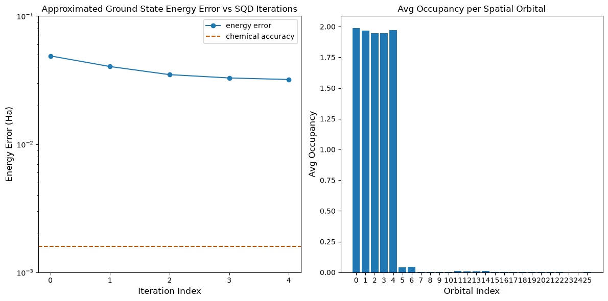
Final energy error: 0.03194368084709254

다음 단계

권장 사항

이 작업에 관심이 있으시다면 다음 자료를 참고해 보세요.

• 페르미온 격자 모델의 샘플 기반 크릴로프 양자 대각화 - 변분 앤사츠 대신 시간 진화 Circuit를 사용하는 관련 튜토리얼
• Dice 솔버로 SQD 화학 워크플로우 확장 - 대각화를 위해 더 효율적인 Dice 소프트웨어를 사용하는 방법을 보여주는 페이지
• SQD 애드온 API 문서 - diagonalize_fermionic_hamiltonian 함수 참조
• 양자 중심 슈퍼컴퓨터에서 정확한 대각화 규모를 초월하는 화학 - 이 튜토리얼의 기반이 된 논문