Pauli 상관관계 인코딩을 통한 max-cut 요구사항 감소

사용 시간 예상: Eagle r3 프로세서 기준 35분 (참고: 이는 추정치이며, 실제 실행 시간은 다를 수 있습니다.)

학습 결과

• 다체(multi‑body) Pauli 문자열이 어떻게 고전 최적화 문제의 다항식 압축을 가능하게 하는지를 포함하여 Pauli 상관관계 인코딩(PCE)의 이론적 원리를 이해합니다.

• 근미래 양자 하드웨어에서 대규모 최적화 작업을 인코딩하고 풀기 위해 실제로 PCE를 구현합니다.

사전 요구사항

• 변분 양자 알고리즘

• QAOA와 max-cut

배경

이 튜토리얼에서는 Pauli 상관관계 인코딩 (PCE) [1]을 소개합니다. PCE는 양자 계산에서 더 높은 효율로 최적화 문제를 Qubit에 인코딩하도록 설계된 접근 방식입니다. PCE는 최적화 문제의 고전 변수를 다체(multi-body) Pauli 행렬 상관관계에 매핑하여 문제의 공간 요구사항을 다항식적으로 압축합니다. PCE를 사용하면 인코딩에 필요한 qubit 수가 줄어들어, 제한된 qubit 자원을 가진 근미래 양자 장치에 특히 유리합니다. 또한, PCE가 본질적으로 바렌 플래토(barren plateau) 문제를 완화하며, 이 현상에 대해 초다항식적 내성을 갖는다는 것이 분석적으로 증명되었습니다. 이러한 내장 기능은 양자 최적화 솔버에서 전례 없는 성능을 가능하게 합니다.

개요

PCE 접근 방식은 아래 [1]의 그림 1에 나타난 것처럼 세 가지 주요 단계로 구성됩니다:

1. 최적화 문제를 Pauli 상관관계 공간으로 인코딩합니다.
2. 양자-고전 최적화 솔버를 사용하여 문제를 풉니다.
3. 해를 원래 최적화 공간으로 디코딩합니다. PCE 접근 방식은 Pauli 상관관계 행렬을 처리할 수 있는 모든 양자 최적화 솔버에 적용 가능합니다. 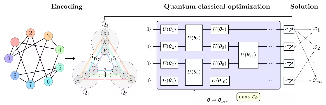[1]의 그림 1에서 max-cut 문제를 PCE 접근 방식을 설명하는 예시로 사용합니다. $m=9$ 노드의 max-cut 문제는 Pauli 상관관계 공간으로 인코딩되어, 최적화 문제를 상관관계 행렬, 구체적으로는 $n=3$ qubit $(Q_1, Q_2, Q_3)$에 걸친 2체(two-body) Pauli 행렬 상관관계로 나타냅니다. 노드의 색상은 각 인코딩된 노드에 사용된 Pauli 문자열을 나타냅니다. 예를 들어, 이진 변수 $x_1$에 해당하는 노드 1은 $Z_1 \otimes Z_2 \otimes I_3$의 기댓값으로 인코딩되며, $x_8$은 $I_1 \otimes Y_2 \otimes Y_3$으로 인코딩됩니다. 이는 문제의 $m$개 변수를 $n = O(m^{1/2})$ Qubit으로 압축하는 것에 해당합니다. 더 일반적으로, $k>1$인 $k$체 상관관계는 $k$차 다항식 압축을 가능하게 합니다. 선택된 Pauli 집합은 상호 가환(mutually-commuting) Pauli 문자열의 세 가지 부분 집합으로 구성되어 있어, 단 세 가지 측정 설정으로 모든 $m$개의 상관관계를 실험적으로 추정할 수 있습니다.

원래 max-cut 목적 함수를 모방하는 Pauli 기댓값의 손실 함수 $\mathcal{L}$이 구성됩니다. 그런 다음, VQE(Variational Quantum Eigensolver)와 같은 양자-고전 최적화 솔버를 사용하여 손실 함수를 최적화합니다.

최적화가 완료되면, 해는 원래 최적화 공간으로 디코딩되어 최적의 max-cut 해를 산출합니다.

요구사항

이 튜토리얼을 시작하기 전에 다음이 설치되어 있는지 확인하세요:

• Qiskit SDK v1.0 이상, 시각화 지원 포함
• Qiskit Runtime v0.22 이상 (pip install qiskit-ibm-runtime)
• Optimization Mapper Qiskit 애드온 (pip install qiskit-addon-opt-mapper)

설정

# Added by doQumentation — installs the packages this notebook needs if they are missing
import importlib.util

_needed = {"networkx": "networkx", "numpy": "numpy", "qiskit": "qiskit", "qiskit_addon_opt_mapper": "qiskit-addon-opt-mapper", "qiskit_aer": "qiskit-aer", "qiskit_ibm_runtime": "qiskit-ibm-runtime", "rustworkx": "rustworkx", "scipy": "scipy"}
_missing = [pip for module, pip in _needed.items()
            if importlib.util.find_spec(module) is None]
# One at a time, so a package that fails to install does not block the others
for _pip in _missing:
    %pip install -q {_pip}
if not _missing:
    print("\u2713 All required packages are installed")

from itertools import combinations

import numpy as np
import rustworkx as rx
import networkx as nx

from scipy.optimize import minimize, OptimizeResult

from qiskit.circuit.library import efficient_su2
from qiskit.transpiler.preset_passmanagers import generate_preset_pass_manager
from qiskit.quantum_info import SparsePauliOp
from qiskit_ibm_runtime import EstimatorV2 as Estimator
from qiskit_ibm_runtime import QiskitRuntimeService
from qiskit_ibm_runtime import Session
from rustworkx.visualization import mpl_draw
from qiskit_aer import AerSimulator

from qiskit_addon_opt_mapper.applications import Maxcut

def make_cut_evaluator(problem):
    """Return a function that maps a 0/1 node assignment to its cut value.

    The objective of the max-cut ``OptimizationProblem`` is the cut value
    itself, and ``problem.objective.evaluate`` computes it for one
    assignment. The swap search in Step 4 evaluates one candidate
    assignment per edge, so pull the objective's coefficients out once
    and evaluate them as a sparse matrix product instead.
    """
    quadratic = problem.objective.quadratic.coefficients.tocsr()
    linear = problem.objective.linear.to_array()
    constant = problem.objective.constant

    def evaluate_cut(bits):
        x = np.asarray(bits, dtype=float)
        return int(round(constant + linear @ x + x @ (quadratic @ x)))

    return evaluate_cut

소규모 시뮬레이터 예제

service = QiskitRuntimeService()
real_backend = service.least_busy(
    operational=True, simulator=False, min_num_qubits=156
)
backend = AerSimulator.from_backend(real_backend)
print(f"We are using the {backend.name}")

We are using the aer_simulator_from(ibm_pittsburgh)

1단계: 고전적 입력을 양자 문제로 매핑하기

max-cut 문제

max-cut 문제는 그래프 $G = (V, E)$에서 정의되는 조합 최적화 문제로, $V$는 꼭짓점의 집합이고 $E$는 간선의 집합입니다. 목표는 두 집합 $S$와 $V \setminus S$ 사이의 간선 수가 최대가 되도록 꼭짓점을 두 집합으로 분할하는 것입니다. max-cut 문제에 대한 자세한 설명은 양자 근사 최적화 알고리즘 튜토리얼을 참조하세요. 또한, max-cut 문제는 QAOA를 위한 고급 기법 튜토리얼에서도 예시로 사용됩니다. 해당 튜토리얼들에서는 QAOA 알고리즘을 사용하여 max-cut 문제를 풉니다.

그래프 → 최적화 문제

먼저 100개의 노드를 가진 무작위 그래프를 살펴보겠습니다.

num_nodes = 100  # Number of nodes in graph
seed = 42
graph = rx.undirected_gnp_random_graph(num_nodes, 0.1, seed=seed)
mpl_draw(graph)

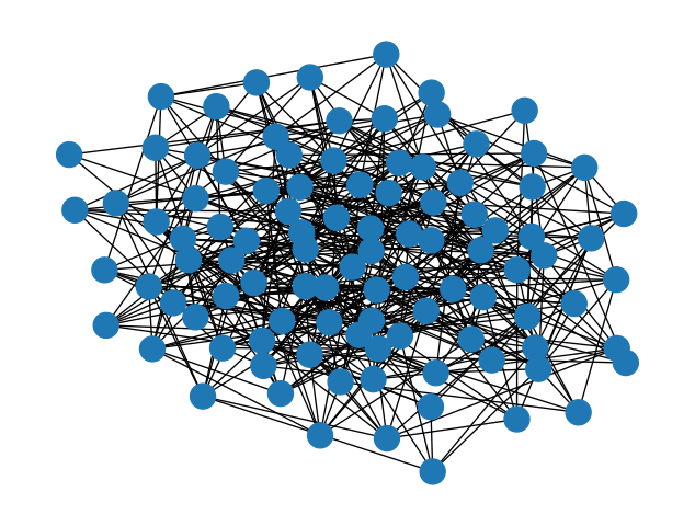
Optimization Mapper Qiskit 애드온의 Maxcut 애플리케이션 클래스로 max-cut 문제를 모델링합니다. 이 클래스는 노드마다 이진 변수 하나를 가지며, 목적 함수가 최대화할 컷 값인 OptimizationProblem을 반환합니다. QAOA 튜토리얼에서는 이 문제를 QUBO로 변환하고 변수당 큐비트 하나를 갖는 비용 해밀토니안으로 변환합니다. 반면 PCE는 각 이진 변수를 파울리 기댓값의 부호로 인코딩하므로, 여기서는 문제가 목적 함수를 정의하고 평가하며 큐비트로의 인코딩은 아래에서 이어집니다.

maxcut = Maxcut(graph)
maxcut_problem = maxcut.to_optimization_problem()
evaluate_cut = make_cut_evaluator(maxcut_problem)

print(f"Binary variables: {maxcut_problem.get_num_vars()}")
print(
    "Quadratic terms (one per edge):",
    len(maxcut_problem.objective.quadratic.to_dict()),
)

Binary variables: 100
Quadratic terms (one per edge): 508

nx_graph = nx.Graph()
nx_graph.add_nodes_from(range(num_nodes))

for edge in graph.edge_list():
    nx_graph.add_edge(edge[0], edge[1])

curr_cut_size, partition = nx.approximation.one_exchange(nx_graph, seed=1)
print(f"Initial cut size: {curr_cut_size}")

Initial cut size: 345

100개의 노드를 가진 그래프를 9개의 Qubit에 걸친 2체 Pauli 행렬 상관관계로 인코딩합니다(아래 설명 참조). 그래프는 상관관계 행렬로 표현되며, 각 노드는 Pauli 문자열로 인코딩됩니다. Pauli 문자열의 기댓값의 부호가 해당 노드의 분할을 나타냅니다. 예를 들어, 노드 0은 Pauli 문자열 $\prod_0 = I_{8} \otimes ... I_2 \otimes X_1 \otimes X_0$으로 인코딩됩니다. 이 Pauli 문자열의 기댓값의 부호가 노드 0의 분할을 나타냅니다. $\prod$에 대한 Pauli 상관관계 인코딩 (PCE)을 다음과 같이 정의합니다:

$x_i \coloneqq \textit{sgn}(\langle\prod_i \rangle),$

여기서 $x_i$는 노드 $i$의 분할이고, $\langle \prod_i \rangle \coloneqq \langle \psi |\prod_i| \psi \rangle$는 양자 상태 $|\psi \rangle$에 대한 노드 $i$를 인코딩하는 Pauli 문자열의 기댓값입니다. 이제 PCE를 사용하여 그래프를 해밀토니안으로 인코딩해 보겠습니다. 노드를 $S_1$, $S_2$, $S_3$ 세 집합으로 나눕니다. 그런 다음, 각 집합의 노드를 각각 $X$, $Y$, $Z$ Pauli 문자열을 사용하여 인코딩합니다. 모든 노드를 인코딩하는 데 필요한 노드 수와 qubit 수 사이의 관계를 구해야 합니다. 인코딩에 가능한 모든 순열을 사용하면 다음과 같습니다:

$$m=3\binom{n}{k}.$$

이 예제에서는 $k=2$를 사용하므로,

$$m = \frac{3}{2} n(n-1).$$

따라서, 특정 노드 수 $m$을 표현하는 데 필요한 qubit 수 $n$은 다음과 같습니다:

$$n = \left\lceil \frac{1 + \sqrt{1 + \tfrac{8}{3}m}}{2} \right\rceil.$$

$\lceil \cdot \rceil$ 기호는 임의의 실수를 다음 정수로 올림하는 천장 함수(ceiling function)를 나타냅니다. 이를 통해 qubit 수가 정수가 됩니다.

num_qubits = int(np.ceil((1 + np.sqrt(1 + (8 / 3) * num_nodes)) / 2))

list_size = num_nodes // 3
node_x = [i for i in range(list_size)]
node_y = [i for i in range(list_size, 2 * list_size)]
node_z = [i for i in range(2 * list_size, num_nodes)]

print(f"Number of qubits: {num_qubits}")
print("List 1:", node_x)
print("List 2:", node_y)
print("List 3:", node_z)

Number of qubits: 9
List 1: [0, 1, 2, 3, 4, 5, 6, 7, 8, 9, 10, 11, 12, 13, 14, 15, 16, 17, 18, 19, 20, 21, 22, 23, 24, 25, 26, 27, 28, 29, 30, 31, 32]
List 2: [33, 34, 35, 36, 37, 38, 39, 40, 41, 42, 43, 44, 45, 46, 47, 48, 49, 50, 51, 52, 53, 54, 55, 56, 57, 58, 59, 60, 61, 62, 63, 64, 65]
List 3: [66, 67, 68, 69, 70, 71, 72, 73, 74, 75, 76, 77, 78, 79, 80, 81, 82, 83, 84, 85, 86, 87, 88, 89, 90, 91, 92, 93, 94, 95, 96, 97, 98, 99]

def build_pauli_correlation_encoding(pauli, node_list, n, k=2):
    pauli_correlation_encoding = []
    for idx, c in enumerate(combinations(range(n), k)):
        if idx >= len(node_list):
            break
        paulis = ["I"] * n
        paulis[c[0]], paulis[c[1]] = pauli, pauli
        pauli_correlation_encoding.append(("".join(paulis)[::-1], 1))

    hamiltonian = []
    for pauli, weight in pauli_correlation_encoding:
        hamiltonian.append(SparsePauliOp.from_list([(pauli, weight)]))

    return hamiltonian

pauli_correlation_encoding_x = build_pauli_correlation_encoding(
    "X", node_x, num_qubits
)
pauli_correlation_encoding_y = build_pauli_correlation_encoding(
    "Y", node_y, num_qubits
)
pauli_correlation_encoding_z = build_pauli_correlation_encoding(
    "Z", node_z, num_qubits
)

2단계: 양자 하드웨어 실행을 위한 문제 최적화

양자 Circuit

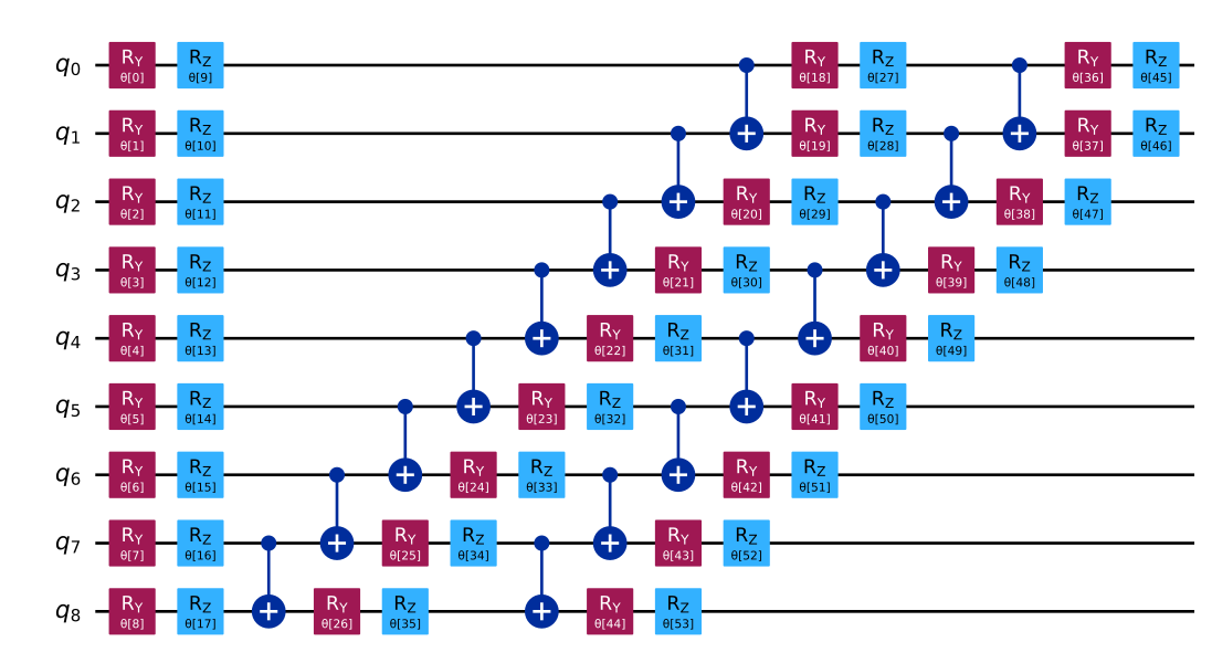
여기서 상태 $|\psi \rangle$는 $\mathbf{\theta}$로 매개변수화되며, 변분 접근 방식을 사용하여 이 매개변수 $\mathbf{\theta}$를 최적화합니다. 이 튜토리얼에서는 표현력과 구현의 용이성으로 인해 변분 알고리즘의 앤사츠(ansatz)로 efficient_su2를 사용합니다. 또한, 이 튜토리얼에서 나중에 소개될 완화된 손실 함수도 사용합니다. 그 결과, 더 적은 Qubit과 얕은 Circuit 깊이로 대규모 문제를 다룰 수 있습니다.

# Build the quantum circuit
qc = efficient_su2(num_qubits, su2_gates=["ry", "rz"], reps=2)
qc.draw("mpl")

# Optimize the circuit

pm = generate_preset_pass_manager(optimization_level=3, backend=backend)
qc = pm.run(qc)

손실 함수

손실 함수 $\mathcal{L}$으로, [1]에 설명된 max-cut 목적 함수의 완화된 형태를 사용합니다. 이는 $\mathcal{V}(\mathbf{x}) \coloneqq \sum_{(i, j) \in E} W_{i, j}(1-x_i x_j)$로 정의됩니다. 여기서 $W_{i, j}$는 간선 $(i, j)$의 가중치를 나타내고, $x_i$는 노드 $i$의 분할을 나타냅니다. 손실 함수 $\mathcal{L}$은 다음과 같이 정의됩니다:

$\mathcal{L}\coloneqq \sum_{(i, j) \in E} W_{i, j} \text{tanh} (\alpha \langle\prod_i \rangle) \text{tanh} (\alpha \langle\prod_j \rangle) + \mathcal{L}^{(\text{reg})}$,

여기서 max-cut 목적 함수는 노드를 인코딩하는 Pauli 문자열의 기댓값에 대한 매끄러운 쌍곡선 탄젠트(hyperbolic tangent)로 대체됩니다. 정규화 항 $\mathcal{L}^{(\text{reg})}$와 qubit 수에 비례하는 재조정 인수 $\alpha$는 솔버의 성능을 향상시키기 위해 도입됩니다.

정규화 항은 다음과 같이 정의됩니다:

$\mathcal{L}^{(\text{reg})}$는 $\mathcal{L}^{(\text{reg})} \coloneqq \beta \nu \lbrack \frac{1}{m} \sum_{i \in V} \text{tanh} (\alpha \langle\prod_i \rangle)^2 \rbrack ^2$으로 정의됩니다.

여기서 $\beta=1/2$, $\nu = |E|/2 + (m -1) /4$이며, $|E|$는 간선의 수이고, $m$은 그래프의 노드 수입니다.

def loss_func_estimator(x, ansatz, hamiltonian, estimator, graph):
    """
    Calculates the specified loss function for the given ansatz, Hamiltonian,
    and graph.

    The expectation values of each Pauli string in the Hamiltonian are first
    obtained by running the ansatz on the quantum backend. These
    expectation values are then passed through the nonlinear function
    tanh(alpha * prod_i). The loss function is
    subsequently computed from these transformed values.
    """
    job = estimator.run(
        [
            (ansatz, hamiltonian[0], x),
            (ansatz, hamiltonian[1], x),
            (ansatz, hamiltonian[2], x),
        ]
    )
    result = job.result()

    # calculate the loss function
    node_exp_map = {}
    idx = 0
    for r in result:
        for ev in r.data.evs:
            node_exp_map[idx] = ev
            idx += 1

    loss = 0
    alpha = num_qubits
    for edge0, edge1 in graph.edge_list():
        loss += np.tanh(alpha * node_exp_map[edge0]) * np.tanh(
            alpha * node_exp_map[edge1]
        )

    regulation_term = 0
    for i in range(len(graph.nodes())):
        regulation_term += np.tanh(alpha * node_exp_map[i]) ** 2
    regulation_term = regulation_term / len(graph.nodes())
    regulation_term = regulation_term**2
    beta = 1 / 2
    v = len(graph.edges()) / 2 + (len(graph.nodes()) - 1) / 4
    regulation_term = beta * v * regulation_term

    loss = loss + regulation_term

    global experiment_result
    print(f"Iter {len(experiment_result)}: {loss}")
    experiment_result.append({"loss": loss, "exp_map": node_exp_map})
    return loss

3단계: Qiskit 프리미티브를 사용하여 실행

이 튜토리얼에서는 시연 목적으로 최적화 루프에 max_iter=50을 설정합니다. 반복 횟수를 늘리면 더 나은 결과를 기대할 수 있습니다.

pce = []
pce.append(
    [op.apply_layout(qc.layout) for op in pauli_correlation_encoding_x]
)
pce.append(
    [op.apply_layout(qc.layout) for op in pauli_correlation_encoding_y]
)
pce.append(
    [op.apply_layout(qc.layout) for op in pauli_correlation_encoding_z]
)

max_iter = 50
counter = {"i": 0}
last_x = {"value": None}
last_fun = {"value": None}

with Session(backend=backend) as session:
    estimator = Estimator(mode=session)

    experiment_result = []

    def loss_func(x):
        last_x["value"] = x.copy()
        if counter["i"] + 1 > max_iter:
            return last_fun["value"]
        counter["i"] += 1
        val = loss_func_estimator(
            x, qc, [pce[0], pce[1], pce[2]], estimator, graph
        )
        last_fun["value"] = val
        return val

    np.random.seed(seed)
    initial_params = np.random.rand(qc.num_parameters)

    result = minimize(
        loss_func, initial_params, method="COBYLA", options={"rhobeg": 1.0}
    )

    if counter["i"] >= max_iter:
        result = OptimizeResult(
            message=f"Return from COBYLA because the objective function "
            f"has been evaluated {max_iter} times.",
            success=False,
            status=3,
            fun=last_fun["value"],
            x=last_x["value"],
            nfev=counter["i"],
        )

print(result)

Iter 0: 152.06331779109445

Iter 1: 126.93132569244693

Iter 2: 55.00651109478942

Iter 3: 33.21667439735082

Iter 4: 19.167189700765054

Iter 5: 30.426875553389127

Iter 6: 13.906354614925815

Iter 7: 27.668686100172614

Iter 8: 28.194600411380772

Iter 9: 24.899677141564936

Iter 10: 22.10858041608358

Iter 11: 8.096210209030176

Iter 12: 8.761240650022913

Iter 13: 9.43332962472133

Iter 14: 7.559669820210062

Iter 15: 13.023860357384214

Iter 16: 11.953653163007987

Iter 17: 10.434221292269214

Iter 18: 4.871246922225549

Iter 19: 10.303826533395856

Iter 20: 16.40225843511339

Iter 21: 10.852469442638652

Iter 22: 9.314666066331633

Iter 23: 6.082358010011717

Iter 24: 10.982893700414476

Iter 25: 4.575556036893407

Iter 26: 6.844995727798197

Iter 27: 8.695229718011293

Iter 28: 3.730227705075576

Iter 29: 4.285479467758721

Iter 30: 4.219714169314187

Iter 31: 0.21125608131726548

Iter 32: 4.22820465672552

Iter 33: 13.67513152473414

Iter 34: 10.388838701884863

Iter 35: -0.5400153834163355

Iter 36: 5.310281742761159

Iter 37: -0.5430772019249082

Iter 38: -4.47820293096989

Iter 39: -3.4832056790567467

Iter 40: -0.5087341672330172

Iter 41: -2.488777859669888

Iter 42: 0.34945469121089356

Iter 43: -0.8544299675507805

Iter 44: -3.5902371208579344

Iter 45: 2.6609573847203216

Iter 46: -4.336467834641085

Iter 47: 0.10158504073828034

Iter 48: -1.3506458813942084

Iter 49: -2.1794894170194192

message: Return from COBYLA because the objective function has been evaluated 50 times.
 success: False
  status: 3
     fun: -2.1794894170194192
       x: [ 1.375e+00  1.951e+00 ...  9.395e-01  8.948e-01]
    nfev: 50

4단계: 결과를 후처리하여 원하는 고전적 형식으로 반환

노드의 분할은 노드를 인코딩하는 파울리 문자열의 기댓값 부호를 평가하여 결정합니다. 기댓값이 0 이상이면 노드에 값 1을 할당하고, 음수이면 0을 할당합니다. 그런 다음 Maxcut의 interpret 메서드가 이 할당을 두 노드 집합으로 디코딩합니다.

# Decode the node assignment from the iteration with the lowest loss.
# If the expectation value is non-negative, the node is assigned 1,
# otherwise it is assigned 0.
def get_bits(experiment_result):
    best_index = min(
        range(len(experiment_result)),
        key=lambda i: experiment_result[i]["loss"],
    )
    exp_map = experiment_result[best_index]["exp_map"]
    bits = [1 if exp_map[i] >= 0 else 0 for i in range(len(exp_map))]
    return bits, best_index

cur_bits, best_index = get_bits(experiment_result)
partition = maxcut.interpret(np.array(cur_bits))
print("Partition 0:", partition[0])
print("Partition 1:", partition[1])

Partition 0: [0, 1, 3, 5, 6, 7, 9, 11, 12, 14, 15, 17, 22, 24, 25, 28, 31, 32, 33, 35, 37, 38, 39, 40, 41, 43, 49, 53, 54, 56, 59, 61, 63, 65, 67, 68, 69, 77, 78, 79, 80, 88, 92, 93, 94, 95]
Partition 1: [2, 4, 8, 10, 13, 16, 18, 19, 20, 21, 23, 26, 27, 29, 30, 34, 36, 42, 44, 45, 46, 47, 48, 50, 51, 52, 55, 57, 58, 60, 62, 64, 66, 70, 71, 72, 73, 74, 75, 76, 81, 82, 83, 84, 85, 86, 87, 89, 90, 91, 96, 97, 98, 99]

이 할당에 대해 OptimizationProblem의 목적 함수를 평가하여 max-cut 문제의 컷 크기를 계산할 수 있습니다.

cut_size = evaluate_cut(cur_bits)
print(f"Cut size: {cut_size}")

Cut size: 278

학습이 완료되면 고전적 후처리 단계로 단일 비트 스왑 탐색을 한 번 수행하여 해를 개선합니다. 이 과정에서 두 노드의 분할을 교환하고 컷 크기를 평가합니다. 컷 크기가 개선되면 교환을 유지합니다. 이 과정을 간선으로 연결된 모든 가능한 노드 쌍에 대해 반복합니다.

# Swap the partitions and calculate the cut size

def swap_partitions(graph, cur_bits, evaluate_cut):
    best_cut = 0
    best_bits = []
    for edge0, edge1 in graph.edge_list():
        swapped_bits = cur_bits.copy()
        swapped_bits[edge0], swapped_bits[edge1] = (
            swapped_bits[edge1],
            swapped_bits[edge0],
        )
        cut_size = evaluate_cut(swapped_bits)
        if best_cut < cut_size:
            best_cut = cut_size
            best_bits = swapped_bits
    return best_cut, best_bits

best_cut, best_bits = swap_partitions(graph, cur_bits, evaluate_cut)
print(best_cut, best_bits)

287 [0, 0, 1, 0, 1, 0, 0, 0, 1, 0, 1, 0, 0, 1, 0, 0, 1, 0, 1, 1, 1, 1, 0, 1, 0, 0, 1, 1, 0, 1, 1, 0, 0, 0, 1, 1, 0, 0, 0, 0, 0, 0, 1, 0, 1, 1, 1, 1, 1, 0, 1, 1, 1, 0, 0, 1, 0, 1, 1, 0, 1, 0, 1, 0, 1, 0, 1, 0, 0, 0, 1, 1, 1, 1, 1, 1, 1, 0, 0, 0, 0, 1, 1, 1, 1, 1, 1, 1, 0, 1, 1, 1, 0, 0, 0, 0, 1, 1, 1, 1]

대규모 하드웨어 예제

# -------------------------Step 1-------------------------

num_nodes = 1500  # Number of nodes in graph
graph = rx.undirected_gnp_random_graph(num_nodes, 0.1, seed=seed)
nx_graph = nx.Graph()
nx_graph.add_nodes_from(range(num_nodes))
for edge in graph.edge_list():
    nx_graph.add_edge(edge[0], edge[1])

maxcut = Maxcut(graph)
maxcut_problem = maxcut.to_optimization_problem()
evaluate_cut = make_cut_evaluator(maxcut_problem)

num_qubits = int(np.ceil((1 + np.sqrt(1 + (8 / 3) * num_nodes)) / 2))

list_size = num_nodes // 3
node_x = [i for i in range(list_size)]
node_y = [i for i in range(list_size, 2 * list_size)]
node_z = [i for i in range(2 * list_size, num_nodes)]

pauli_correlation_encoding_x = build_pauli_correlation_encoding(
    "X", node_x, num_qubits
)
pauli_correlation_encoding_y = build_pauli_correlation_encoding(
    "Y", node_y, num_qubits
)
pauli_correlation_encoding_z = build_pauli_correlation_encoding(
    "Z", node_z, num_qubits
)
print(f"We are using {num_qubits} qubits")

# -------------------------Step 2-------------------------
backend = real_backend
print(f"We are using the {backend.name}")
qc = efficient_su2(num_qubits, ["ry", "rz"], reps=2)
pm = generate_preset_pass_manager(optimization_level=3, backend=backend)
qc = pm.run(qc)
# -------------------------Step 3-------------------------
pce = []
pce.append(
    [op.apply_layout(qc.layout) for op in pauli_correlation_encoding_x]
)
pce.append(
    [op.apply_layout(qc.layout) for op in pauli_correlation_encoding_y]
)
pce.append(
    [op.apply_layout(qc.layout) for op in pauli_correlation_encoding_z]
)

# Run the optimization using a session.
max_iter = 50
counter = {"i": 0}
with Session(backend=backend) as session:
    estimator = Estimator(mode=session)
    estimator.options.environment.job_tags = ["TUT_PCEFQ"]
    experiment_result = []

    def loss_func(x):
        last_x["value"] = x.copy()
        if counter["i"] + 1 > max_iter:
            return last_fun["value"]
        counter["i"] += 1
        val = loss_func_estimator(
            x, qc, [pce[0], pce[1], pce[2]], estimator, graph
        )
        last_fun["value"] = val
        return val

    np.random.seed(seed)
    initial_params = np.random.rand(qc.num_parameters)
    result = minimize(
        loss_func, initial_params, method="COBYLA", options={"rhobeg": 1.0}
    )
    if counter["i"] >= max_iter:
        result = OptimizeResult(
            message=f"Return from COBYLA because the objective function "
            f"has been evaluated {max_iter} times.",
            success=False,
            status=3,
            fun=last_fun["value"],
            x=last_x["value"],
            nfev=counter["i"],
        )
print(result)

# -------------------------Step 4-------------------------

cur_bits, best_index = get_bits(experiment_result)
cut_size = evaluate_cut(cur_bits)
print(f"Cut size: {cut_size}")

best_cut, best_bits = swap_partitions(graph, cur_bits, evaluate_cut)
# Print final solution

print(
    f"The best max-cut value achieved for a graph with {num_nodes} nodes "
    f"on {num_qubits} qubits is {best_cut}"
)
print(f"and the specific partition we obtained is {best_bits}")

We are using 33 qubits
We are using the ibm_pittsburgh

Iter 0: 62192.56098951446

Iter 1: 54325.76340818571

Iter 2: 42933.215216568526

Iter 3: 35721.92960658595

Iter 4: 35947.69927402131

Iter 5: 38563.731543582166

Iter 6: 32552.97070835923

Iter 7: 34730.314616527576

Iter 8: 27032.920190652876

Iter 9: 27126.107795624957

Iter 10: 25268.853826648774

Iter 11: 23521.1489346676

Iter 12: 21658.585394613096

Iter 13: 15154.765728388778

Iter 14: 14826.985321939152

Iter 15: 16199.811009055386

Iter 16: 14328.589985020852

Iter 17: 13542.67789354434

Iter 18: 11737.341026421902

Iter 19: 10986.431644208033

Iter 20: 9780.61657788984

Iter 21: 8555.757154943312

Iter 22: 10465.489221259657

Iter 23: 8577.158776664453

Iter 24: 8950.176436175909

Iter 25: 7395.8803219317215

Iter 26: 7228.1129297581765

Iter 27: 6881.076354027118

Iter 28: 6626.8983738084835

Iter 29: 7302.433279572058

Iter 30: 6995.735525608492

Iter 31: 6176.828001182083

Iter 32: 6299.8061884979725

Iter 33: 6498.921256598082

Iter 34: 6184.684072713035

Iter 35: 5707.720358527108

Iter 36: 5414.328928670104

Iter 37: 5771.80573980932

Iter 38: 5620.64903695431

Iter 39: 6285.735849503706

Iter 40: 5894.367571492991

Iter 41: 6079.275064349491

Iter 42: 5267.448536682269

Iter 43: 4789.7281459863325

Iter 44: 5109.106057200384

Iter 45: 5060.248865782273

Iter 46: 5064.786713246322

Iter 47: 5474.433264995371

Iter 48: 4675.6138719238015

Iter 49: 5081.660754434205

message: Return from COBYLA because the objective function has been evaluated 50 times.
 success: False
  status: 3
     fun: 5081.660754434205
       x: [ 1.375e+00  1.951e+00 ...  7.260e-01  8.971e-01]
    nfev: 50
Cut size: 55507

The best max-cut value achieved for a graph with 1500 nodes on 33 qubits is 55567
and the specific partition we obtained is [1, 0, 0, 1, 1, 1, 1, 0, 0, 1, 1, 1, 0, 1, 0, 1, 0, 0, 0, 1, 1, 0, 1, 0, 0, 1, 1, 0, 0, 1, 1, 1, 0, 0, 0, 0, 0, 1, 0, 0, 0, 1, 1, 1, 1, 0, 0, 0, 0, 1, 0, 0, 0, 0, 1, 1, 1, 0, 1, 1, 1, 0, 1, 0, 0, 0, 0, 0, 0, 1, 0, 1, 1, 0, 0, 1, 1, 1, 1, 0, 1, 0, 1, 1, 0, 1, 1, 0, 0, 0, 1, 1, 1, 0, 1, 1, 0, 0, 1, 0, 0, 0, 1, 1, 1, 1, 1, 1, 1, 1, 0, 0, 0, 1, 1, 1, 1, 1, 1, 0, 0, 0, 1, 1, 0, 1, 0, 1, 0, 1, 0, 1, 1, 1, 0, 0, 0, 0, 1, 0, 0, 0, 0, 0, 0, 0, 1, 0, 1, 1, 1, 0, 1, 0, 1, 0, 1, 0, 0, 0, 1, 0, 0, 0, 0, 1, 0, 0, 1, 1, 1, 1, 1, 1, 1, 1, 1, 1, 1, 0, 1, 0, 0, 0, 0, 0, 0, 0, 1, 0, 1, 1, 1, 1, 1, 1, 1, 1, 1, 1, 0, 1, 1, 0, 0, 0, 0, 0, 0, 0, 0, 0, 0, 0, 1, 1, 0, 0, 0, 0, 0, 1, 0, 0, 0, 0, 0, 1, 0, 1, 0, 0, 0, 0, 1, 0, 1, 1, 1, 1, 1, 0, 1, 1, 0, 0, 1, 1, 1, 0, 1, 1, 1, 1, 0, 1, 0, 1, 1, 0, 1, 1, 1, 0, 0, 0, 0, 1, 1, 1, 1, 0, 0, 1, 1, 1, 1, 1, 1, 1, 1, 0, 1, 0, 0, 0, 0, 1, 0, 0, 0, 1, 1, 1, 0, 1, 1, 0, 1, 1, 1, 1, 1, 1, 1, 1, 1, 0, 0, 1, 1, 0, 0, 0, 1, 0, 1, 0, 0, 1, 0, 1, 1, 1, 0, 0, 1, 1, 1, 1, 1, 0, 1, 0, 0, 1, 0, 1, 1, 1, 1, 1, 0, 1, 1, 1, 0, 1, 1, 1, 1, 0, 0, 1, 1, 1, 1, 1, 1, 1, 0, 1, 0, 0, 1, 0, 1, 0, 0, 0, 0, 0, 1, 0, 0, 1, 0, 0, 1, 1, 1, 0, 1, 1, 1, 1, 0, 1, 1, 1, 1, 0, 1, 1, 0, 1, 1, 1, 1, 1, 1, 1, 1, 1, 0, 0, 1, 1, 1, 0, 0, 0, 1, 1, 0, 1, 0, 1, 0, 1, 0, 1, 0, 1, 0, 0, 0, 0, 1, 1, 1, 1, 1, 1, 1, 1, 0, 1, 0, 0, 0, 1, 0, 0, 0, 1, 0, 0, 1, 1, 1, 0, 0, 0, 0, 1, 0, 1, 0, 1, 1, 1, 1, 1, 0, 1, 0, 1, 1, 0, 1, 1, 1, 1, 0, 1, 0, 1, 0, 1, 1, 1, 0, 1, 1, 1, 1, 1, 1, 0, 1, 1, 1, 1, 0, 1, 1, 1, 1, 0, 0, 1, 1, 1, 0, 0, 1, 0, 1, 1, 0, 1, 1, 1, 1, 0, 0, 1, 0, 1, 0, 1, 1, 1, 1, 0, 1, 0, 0, 1, 0, 1, 1, 1, 0, 0, 0, 1, 1, 0, 0, 1, 0, 1, 1, 1, 1, 1, 0, 1, 0, 0, 0, 0, 1, 0, 1, 0, 1, 0, 0, 0, 1, 0, 0, 0, 0, 1, 0, 0, 0, 1, 0, 1, 1, 1, 0, 1, 1, 1, 1, 0, 0, 0, 0, 0, 1, 0, 1, 0, 1, 1, 1, 1, 0, 0, 1, 1, 0, 0, 0, 1, 1, 1, 1, 1, 1, 0, 0, 1, 0, 0, 1, 0, 0, 0, 0, 0, 0, 1, 0, 1, 1, 1, 1, 1, 0, 1, 0, 1, 1, 1, 1, 0, 1, 0, 0, 1, 1, 1, 1, 0, 1, 1, 1, 1, 0, 1, 1, 0, 1, 0, 0, 1, 0, 1, 1, 1, 0, 0, 0, 1, 1, 0, 1, 1, 1, 1, 1, 1, 1, 1, 1, 1, 1, 1, 0, 0, 0, 1, 1, 0, 0, 0, 1, 1, 1, 1, 1, 1, 0, 0, 1, 0, 1, 1, 0, 0, 0, 0, 0, 0, 0, 0, 1, 0, 1, 0, 1, 0, 0, 0, 1, 1, 0, 0, 0, 0, 1, 1, 1, 1, 1, 0, 1, 1, 0, 1, 0, 1, 1, 1, 0, 1, 1, 1, 0, 1, 0, 1, 1, 1, 1, 0, 1, 1, 1, 1, 1, 1, 1, 1, 0, 0, 0, 0, 0, 0, 0, 1, 0, 0, 0, 0, 0, 0, 1, 0, 1, 0, 1, 0, 0, 0, 1, 0, 1, 0, 1, 0, 1, 0, 0, 0, 1, 0, 1, 1, 1, 0, 1, 1, 0, 0, 1, 1, 0, 1, 1, 0, 1, 1, 1, 1, 1, 1, 0, 0, 1, 1, 0, 1, 1, 1, 1, 1, 1, 0, 0, 1, 1, 1, 0, 0, 0, 0, 0, 1, 1, 1, 0, 1, 1, 0, 1, 0, 1, 0, 0, 1, 1, 1, 1, 1, 1, 0, 0, 0, 1, 1, 0, 0, 1, 0, 1, 1, 0, 0, 0, 1, 0, 0, 0, 0, 1, 1, 0, 1, 0, 1, 0, 1, 0, 0, 1, 0, 1, 1, 1, 0, 1, 0, 1, 1, 1, 1, 1, 0, 1, 0, 1, 0, 0, 1, 0, 1, 0, 1, 0, 1, 0, 0, 0, 1, 0, 0, 1, 0, 0, 1, 0, 1, 0, 0, 0, 0, 1, 1, 0, 1, 0, 1, 0, 0, 1, 1, 1, 0, 1, 1, 1, 1, 0, 1, 0, 1, 0, 0, 1, 0, 0, 1, 0, 1, 1, 0, 0, 1, 0, 1, 0, 1, 0, 1, 1, 1, 0, 1, 0, 0, 1, 0, 0, 0, 0, 0, 1, 1, 1, 0, 1, 1, 0, 1, 0, 1, 0, 1, 1, 1, 0, 0, 0, 1, 1, 1, 1, 1, 1, 1, 1, 0, 1, 1, 1, 1, 1, 0, 1, 0, 0, 0, 0, 1, 1, 1, 1, 1, 1, 1, 1, 0, 1, 0, 1, 1, 1, 1, 0, 1, 1, 1, 1, 0, 1, 1, 1, 1, 1, 1, 1, 1, 0, 1, 0, 0, 0, 1, 0, 1, 0, 0, 1, 1, 1, 1, 0, 0, 1, 0, 0, 0, 1, 0, 0, 1, 0, 0, 0, 1, 1, 0, 1, 1, 0, 0, 0, 1, 0, 0, 0, 0, 0, 1, 0, 1, 0, 1, 0, 0, 1, 0, 0, 0, 0, 1, 0, 0, 0, 0, 0, 0, 0, 0, 0, 0, 1, 0, 1, 0, 0, 0, 0, 1, 0, 0, 0, 1, 0, 1, 0, 1, 0, 0, 0, 0, 0, 0, 0, 1, 0, 0, 1, 1, 0, 1, 1, 1, 0, 1, 0, 0, 0, 1, 1, 1, 1, 1, 1, 1, 1, 1, 0, 1, 1, 1, 0, 0, 1, 0, 1, 0, 1, 0, 1, 1, 0, 0, 0, 1, 1, 1, 1, 1, 1, 1, 1, 1, 1, 0, 1, 1, 1, 1, 0, 1, 0, 0, 1, 1, 1, 1, 0, 0, 0, 1, 1, 1, 1, 1, 1, 1, 1, 1, 1, 0, 1, 1, 1, 1, 1, 1, 0, 0, 1, 0, 0, 0, 1, 0, 1, 0, 0, 0, 0, 0, 0, 1, 0, 0, 0, 0, 0, 0, 1, 0, 0, 0, 0, 1, 0, 0, 0, 0, 1, 1, 0, 1, 1, 1, 1, 1, 1, 1, 0, 1, 1, 1, 1, 1, 1, 0, 1, 1, 1, 0, 0, 0, 1, 1, 1, 0, 0, 1, 1, 1, 0, 1, 1, 1, 0, 1, 1, 1, 1, 0, 0, 0, 1, 0, 1, 1, 0, 1, 1, 1, 1, 1, 1, 1, 1, 1, 1, 1, 0, 1, 0, 1, 0, 0, 0, 1, 1, 1, 1, 0, 0, 0, 1, 0, 0, 0, 0, 0, 1, 0, 1, 0, 1, 1, 1, 0, 0, 1, 0, 1, 1, 1, 0, 0, 1, 0, 0, 0, 0, 1, 0, 1, 1, 0, 0, 1, 0, 0, 0, 0, 0, 0, 0, 0, 0, 0, 0, 0, 0, 0, 0, 1, 0, 0, 1, 0, 0, 0, 0, 0, 0, 1, 0, 0, 0, 0, 0, 0, 0, 1, 1, 1, 0, 1, 1, 0, 1, 0, 1, 1, 1, 1, 1, 1, 1, 0, 1, 1, 0, 1, 1, 1, 1, 1, 1, 1, 1, 1, 1, 0, 1, 0, 1, 1, 0, 1, 0, 1, 1, 0, 1, 0, 1, 1, 1, 1, 0, 1, 1, 0, 0, 0, 0, 1, 0, 1, 0, 0, 0, 0, 0, 1, 1, 0, 1, 0, 0, 1, 1, 1, 0, 0, 1, 0, 1, 0, 1, 1, 0, 1, 0, 1, 1, 1, 1, 1, 0, 1, 1, 1, 1, 1, 1, 1, 1, 1, 0, 1, 1, 1, 0, 1, 1, 1, 1, 1, 1, 1, 1, 1, 1, 1, 1, 1, 1, 0, 1, 1, 0, 1, 1, 1, 1, 1]

다음 단계

Recommendations

이 작업이 흥미로우셨다면 다음 자료도 참고해 보세요:

• QAOA를 위한 고급 기법
• Estimator 프리미티브로 오류 완화 옵션 결합하기

참고문헌

[1] Sciorilli, M., Borges, L., Patti, T. L., García-Martín, D., Camilo, G., Anandkumar, A., & Aolita, L. (2024). Towards large-scale quantum optimization solvers with few qubits. arXiv preprint arXiv:2401.09421.

튜토리얼 설문조사

이 튜토리얼에 대한 피드백을 제공하기 위해 짧은 설문조사에 참여해 주세요. 여러분의 의견은 콘텐츠 품질과 사용자 경험 개선에 도움이 됩니다.

참고: 이 설문조사는 IBM Quantum에서 진행하며 IBM이 작성한 튜토리얼 콘텐츠를 다룹니다. doQumentation은 웹사이트, 번역, 코드 실행을 제공합니다 — 이에 대한 피드백은 GitHub 이슈를 열어 주세요.

설문조사 링크 © IBM Corp. 2024-2026