격자 해밀토니안의 Krylov 양자 대각화

사용 시간 예상: Heron r2에서 20분 (참고: 이는 예상치이며, 실제 실행 시간은 다를 수 있습니다.)

# Added by doQumentation — required packages for this notebook
!pip install -q matplotlib numpy qiskit qiskit-ibm-runtime scipy sympy

# This cell is hidden from users – it disables some lint rules
# ruff: noqa: E402 E722 F601

배경

이 튜토리얼은 Qiskit 패턴의 맥락에서 Krylov 양자 대각화 알고리즘(KQD)을 구현하는 방법을 설명합니다. 먼저 알고리즘의 이론적 배경을 학습한 후, QPU에서의 실행 데모를 확인할 수 있습니다.

다양한 분야에서 양자 시스템의 바닥 상태 특성을 파악하는 것이 중요합니다. 입자와 힘의 근본적인 성질을 이해하고, 복잡한 물질의 동작을 예측·이해하며, 생화학적 상호작용과 반응을 이해하는 것이 그 예입니다. 힐베르트 공간의 지수적 증가와 얽힌 시스템에서 발생하는 상관관계로 인해, 고전 알고리즘은 규모가 커지는 양자 시스템에서 이 문제를 풀기 어렵습니다. 한쪽 극단에는 양자 하드웨어를 활용하는 기존 방식인 변분 양자 방법(예: 변분 양자 고유값 분해기)이 있습니다. 이 기법들은 최적화 과정에서 많은 함수 호출이 필요하고, 고급 오류 완화 기법을 적용하면 리소스 오버헤드가 커져 소규모 시스템에서만 효과적이라는 한계가 있습니다. 반대쪽 극단에는 성능 보장이 있는 내결함성 양자 방법(예: 양자 위상 추정)이 있으며, 이는 내결함성 장치에서만 실행 가능한 깊은 Circuit을 요구합니다. 이러한 이유로, 여기서는 부분 공간 방법(이 리뷰 논문 참조)에 기반한 양자 알고리즘인 Krylov 양자 대각화(KQD) 알고리즘을 소개합니다. 이 알고리즘은 기존 양자 하드웨어에서 대규모[1]로 잘 작동하며, 위상 추정과 유사한 성능 보장을 갖추고, 고급 오류 완화 기법과 호환되며, 고전적으로는 접근하기 어려운 결과를 제공할 수 있습니다.

요구 사항

이 튜토리얼을 시작하기 전에 다음이 설치되어 있는지 확인하세요:

• Qiskit SDK v2.0 이상(시각화 지원 포함)
• Qiskit Runtime v0.22 이상 ( pip install qiskit-ibm-runtime )

설정

import numpy as np
import scipy as sp
import matplotlib.pylab as plt
from typing import Union, List
import itertools as it
import copy
from sympy import Matrix
import warnings

warnings.filterwarnings("ignore")

from qiskit.quantum_info import SparsePauliOp, Pauli, StabilizerState
from qiskit.circuit import Parameter, IfElseOp
from qiskit import QuantumCircuit, QuantumRegister
from qiskit.circuit.library import PauliEvolutionGate
from qiskit.synthesis import LieTrotter
from qiskit.transpiler import Target, CouplingMap
from qiskit.transpiler.preset_passmanagers import generate_preset_pass_manager

from qiskit_ibm_runtime import (
    QiskitRuntimeService,
    EstimatorV2 as Estimator,
)

def solve_regularized_gen_eig(
    h: np.ndarray,
    s: np.ndarray,
    threshold: float,
    k: int = 1,
    return_dimn: bool = False,
) -> Union[float, List[float]]:
    """
    Method for solving the generalized eigenvalue problem with regularization

    Args:
        h (numpy.ndarray):
            The effective representation of the matrix in the Krylov subspace
        s (numpy.ndarray):
            The matrix of overlaps between vectors of the Krylov subspace
        threshold (float):
            Cut-off value for the eigenvalue of s
        k (int):
            Number of eigenvalues to return
        return_dimn (bool):
            Whether to return the size of the regularized subspace

    Returns:
        lowest k-eigenvalue(s) that are the solution of the regularized generalized eigenvalue problem

    """
    s_vals, s_vecs = sp.linalg.eigh(s)
    s_vecs = s_vecs.T
    good_vecs = np.array(
        [vec for val, vec in zip(s_vals, s_vecs) if val > threshold]
    )
    h_reg = good_vecs.conj() @ h @ good_vecs.T
    s_reg = good_vecs.conj() @ s @ good_vecs.T
    if k == 1:
        if return_dimn:
            return sp.linalg.eigh(h_reg, s_reg)[0][0], len(good_vecs)
        else:
            return sp.linalg.eigh(h_reg, s_reg)[0][0]
    else:
        if return_dimn:
            return sp.linalg.eigh(h_reg, s_reg)[0][:k], len(good_vecs)
        else:
            return sp.linalg.eigh(h_reg, s_reg)[0][:k]

def single_particle_gs(H_op, n_qubits):
    """
    Find the ground state of the single particle(excitation) sector
    """
    H_x = []
    for p, coeff in H_op.to_list():
        H_x.append(set([i for i, v in enumerate(Pauli(p).x) if v]))

    H_z = []
    for p, coeff in H_op.to_list():
        H_z.append(set([i for i, v in enumerate(Pauli(p).z) if v]))

    H_c = H_op.coeffs

    print("n_sys_qubits", n_qubits)

    n_exc = 1
    sub_dimn = int(sp.special.comb(n_qubits + 1, n_exc))
    print("n_exc", n_exc, ", subspace dimension", sub_dimn)

    few_particle_H = np.zeros((sub_dimn, sub_dimn), dtype=complex)

    sparse_vecs = [
        set(vec) for vec in it.combinations(range(n_qubits + 1), r=n_exc)
    ]  # list all of the possible sets of n_exc indices of 1s in n_exc-particle states

    m = 0
    for i, i_set in enumerate(sparse_vecs):
        for j, j_set in enumerate(sparse_vecs):
            m += 1

            if len(i_set.symmetric_difference(j_set)) <= 2:
                for p_x, p_z, coeff in zip(H_x, H_z, H_c):
                    if i_set.symmetric_difference(j_set) == p_x:
                        sgn = ((-1j) ** len(p_x.intersection(p_z))) * (
                            (-1) ** len(i_set.intersection(p_z))
                        )
                    else:
                        sgn = 0

                    few_particle_H[i, j] += sgn * coeff

    gs_en = min(np.linalg.eigvalsh(few_particle_H))
    print("single particle ground state energy: ", gs_en)
    return gs_en

1단계: 고전적 입력을 양자 문제로 매핑하기

크릴로프 공간

차수 $r$의 크릴로프 공간 $\mathcal{K}^r$은 행렬 $A$의 거듭제곱(최대 $r-1$)을 기준 벡터 $\vert v \rangle$에 곱하여 얻은 벡터들로 생성되는 공간입니다.

$$\mathcal{K}^r = \left\{ \vert v \rangle, A \vert v \rangle, A^2 \vert v \rangle, ..., A^{r-1} \vert v \rangle \right\}$$

행렬 $A$가 해밀토니안 $H$인 경우, 대응하는 공간을 거듭제곱 크릴로프 공간 $\mathcal{K}_P$라고 합니다. $A$가 해밀토니안에 의해 생성되는 시간 진화 연산자 $U=e^{-iHt}$인 경우에는 이를 유니터리 크릴로프 공간 $\mathcal{K}_U$라고 합니다. 고전적으로 사용하는 거듭제곱 크릴로프 부분공간은 $H$가 유니터리 연산자가 아니기 때문에 양자 컴퓨터에서 직접 생성할 수 없습니다. 대신 시간 진화 연산자 $U = e^{-iHt}$를 사용할 수 있으며, 이는 거듭제곱 방법과 유사한 수렴 보장을 제공하는 것으로 알려져 있습니다. 이때 $U$의 거듭제곱은 서로 다른 시간 스텝 $U^k = e^{-iH(kt)}$가 됩니다.

$$\mathcal{K}_U^r = \left\{ \vert \psi \rangle, U \vert \psi \rangle, U^2 \vert \psi \rangle, ..., U^{r-1} \vert \psi \rangle \right\}$$

유니터리 크릴로프 공간이 어떻게 저에너지 고유상태를 정확하게 표현하는지에 대한 자세한 유도는 부록을 참고하세요.

크릴로프 양자 대각화 알고리즘

대각화하려는 해밀토니안 $H$가 주어지면, 먼저 대응하는 유니터리 크릴로프 공간 $\mathcal{K}_U$를 고려합니다. 목표는 $\mathcal{K}_U$ 내에서 해밀토니안의 간결한 표현을 찾는 것이며, 이를 $\tilde{H}$라고 부릅니다. 크릴로프 공간에 투영된 해밀토니안 $\tilde{H}$의 행렬 원소들은 다음 기댓값을 계산함으로써 구할 수 있습니다.

$$\tilde{H}_{mn} = \langle \psi_m \vert H \vert \psi_n \rangle =$$ $$= \langle \psi \vert e^{i H t_m} H e^{-i H t_n} \vert \psi \rangle$$ $$= \langle \psi \vert e^{i H m dt} H e^{-i H n dt} \vert \psi \rangle$$

여기서 $\vert \psi_n \rangle = e^{-i H t_n} \vert \psi \rangle$은 유니터리 크릴로프 공간의 벡터들이고, $t_n = n dt$는 선택한 시간 스텝 $dt$의 배수입니다. 양자 컴퓨터에서 각 행렬 원소의 계산은 양자 상태 간의 겹침(overlap)을 구할 수 있는 임의의 알고리즘을 사용할 수 있습니다. 이 튜토리얼에서는 아다마르 테스트(Hadamard test)에 초점을 맞춥니다. $\mathcal{K}_U$의 차원이 $r$이면, 부분공간에 투영된 해밀토니안의 크기는 $r \times r$이 됩니다. $r$이 충분히 작은 경우(일반적으로 고유에너지 추정치의 수렴을 얻기 위해 $r<<100$으로도 충분합니다), 투영된 해밀토니안 $\tilde{H}$를 쉽게 대각화할 수 있습니다. 그러나 크릴로프 공간 벡터들의 비직교성 때문에 $\tilde{H}$를 직접 대각화할 수는 없습니다. 이들의 겹침을 측정하여 행렬 $\tilde{S}$를 구성해야 합니다.

$$\tilde{S}_{mn} = \langle \psi_m \vert \psi_n \rangle$$

이를 통해 비직교 공간에서의 고유값 문제(일반화 고유값 문제라고도 합니다)를 풀 수 있습니다.

$$\tilde{H} \ \vec{c} = E \ \tilde{S} \ \vec{c}$$

이를 통해 $\tilde{H}$의 고유값과 고유상태를 살펴봄으로써 $H$의 고유값과 고유상태에 대한 추정치를 얻을 수 있습니다. 예를 들어, 바닥 상태 에너지의 추정치는 가장 작은 고유값 $c$를 취하고, 대응하는 고유벡터 $\vec{c}$로부터 바닥 상태를 구하는 방식으로 얻습니다. $\vec{c}$의 계수들은 $\mathcal{K}_U$를 생성하는 서로 다른 벡터들의 기여도를 결정합니다.

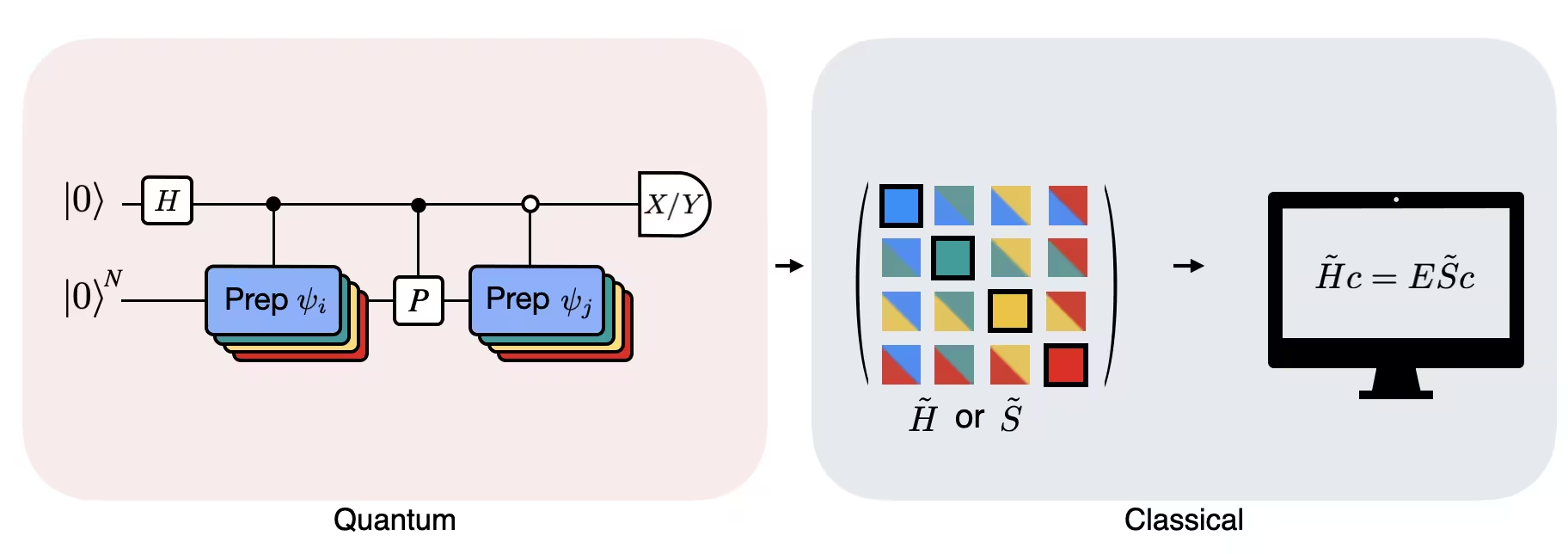
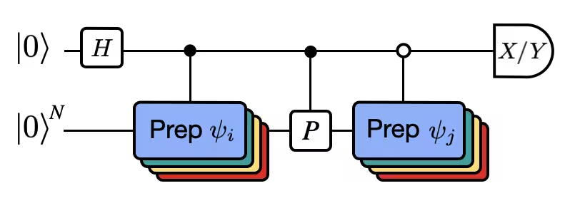
이 그림은 수정된 아다마르 테스트의 Circuit 표현을 보여줍니다. 아다마르 테스트는 서로 다른 양자 상태 간의 겹침을 계산하는 데 사용되는 방법입니다. 각 행렬 원소 $\tilde{H}_{i,j}$에 대해, 상태 $\vert \psi_i \rangle$와 $\vert \psi_j \rangle$ 사이의 아다마르 테스트가 수행됩니다. 이는 행렬 원소의 색상 체계와 대응하는 $\text{Prep} \; \psi_i$, $\text{Prep} \; \psi_j$ 연산으로 그림에 강조되어 있습니다. 따라서 투영된 해밀토니안 $\tilde{H}$의 모든 행렬 원소를 계산하려면 크릴로프 공간 벡터들의 가능한 모든 조합에 대한 아다마르 테스트 세트가 필요합니다. 아다마르 테스트 Circuit에서 위쪽 선은 X 또는 Y 기저에서 측정되는 보조(ancilla) Qubit이며, 그 기댓값이 상태 간 겹침의 값을 결정합니다. 아래쪽 선은 시스템 해밀토니안의 모든 Qubit을 나타냅니다. $\text{Prep} \; \psi_i$ 연산은 보조 Qubit의 상태에 의해 제어되어 시스템 Qubit을 상태 $\vert \psi_i \rangle$로 준비시키며($\text{Prep} \; \psi_j$도 마찬가지입니다), 연산 $P$는 시스템 해밀토니안 $H = \sum_i P_i$의 파울리 분해를 나타냅니다. 아다마르 테스트가 계산하는 연산에 대한 더 자세한 유도는 아래에 나와 있습니다.

해밀토니안 정의

선형 체인 위의 $N$ Qubit에 대한 하이젠베르크 해밀토니안을 고려해 봅시다: $H= \sum_{i,j}^N X_i X_j + Y_i Y_j - J Z_i Z_j$

# Define problem Hamiltonian.
n_qubits = 30
J = 1  # coupling strength for ZZ interaction

# Define the Hamiltonian:
H_int = [["I"] * n_qubits for _ in range(3 * (n_qubits - 1))]
for i in range(n_qubits - 1):
    H_int[i][i] = "Z"
    H_int[i][i + 1] = "Z"
for i in range(n_qubits - 1):
    H_int[n_qubits - 1 + i][i] = "X"
    H_int[n_qubits - 1 + i][i + 1] = "X"
for i in range(n_qubits - 1):
    H_int[2 * (n_qubits - 1) + i][i] = "Y"
    H_int[2 * (n_qubits - 1) + i][i + 1] = "Y"
H_int = ["".join(term) for term in H_int]
H_tot = [(term, J) if term.count("Z") == 2 else (term, 1) for term in H_int]

# Get operator
H_op = SparsePauliOp.from_list(H_tot)
print(H_tot)

[('ZZIIIIIIIIIIIIIIIIIIIIIIIIIIII', 1), ('IZZIIIIIIIIIIIIIIIIIIIIIIIIIII', 1), ('IIZZIIIIIIIIIIIIIIIIIIIIIIIIII', 1), ('IIIZZIIIIIIIIIIIIIIIIIIIIIIIII', 1), ('IIIIZZIIIIIIIIIIIIIIIIIIIIIIII', 1), ('IIIIIZZIIIIIIIIIIIIIIIIIIIIIII', 1), ('IIIIIIZZIIIIIIIIIIIIIIIIIIIIII', 1), ('IIIIIIIZZIIIIIIIIIIIIIIIIIIIII', 1), ('IIIIIIIIZZIIIIIIIIIIIIIIIIIIII', 1), ('IIIIIIIIIZZIIIIIIIIIIIIIIIIIII', 1), ('IIIIIIIIIIZZIIIIIIIIIIIIIIIIII', 1), ('IIIIIIIIIIIZZIIIIIIIIIIIIIIIII', 1), ('IIIIIIIIIIIIZZIIIIIIIIIIIIIIII', 1), ('IIIIIIIIIIIIIZZIIIIIIIIIIIIIII', 1), ('IIIIIIIIIIIIIIZZIIIIIIIIIIIIII', 1), ('IIIIIIIIIIIIIIIZZIIIIIIIIIIIII', 1), ('IIIIIIIIIIIIIIIIZZIIIIIIIIIIII', 1), ('IIIIIIIIIIIIIIIIIZZIIIIIIIIIII', 1), ('IIIIIIIIIIIIIIIIIIZZIIIIIIIIII', 1), ('IIIIIIIIIIIIIIIIIIIZZIIIIIIIII', 1), ('IIIIIIIIIIIIIIIIIIIIZZIIIIIIII', 1), ('IIIIIIIIIIIIIIIIIIIIIZZIIIIIII', 1), ('IIIIIIIIIIIIIIIIIIIIIIZZIIIIII', 1), ('IIIIIIIIIIIIIIIIIIIIIIIZZIIIII', 1), ('IIIIIIIIIIIIIIIIIIIIIIIIZZIIII', 1), ('IIIIIIIIIIIIIIIIIIIIIIIIIZZIII', 1), ('IIIIIIIIIIIIIIIIIIIIIIIIIIZZII', 1), ('IIIIIIIIIIIIIIIIIIIIIIIIIIIZZI', 1), ('IIIIIIIIIIIIIIIIIIIIIIIIIIIIZZ', 1), ('XXIIIIIIIIIIIIIIIIIIIIIIIIIIII', 1), ('IXXIIIIIIIIIIIIIIIIIIIIIIIIIII', 1), ('IIXXIIIIIIIIIIIIIIIIIIIIIIIIII', 1), ('IIIXXIIIIIIIIIIIIIIIIIIIIIIIII', 1), ('IIIIXXIIIIIIIIIIIIIIIIIIIIIIII', 1), ('IIIIIXXIIIIIIIIIIIIIIIIIIIIIII', 1), ('IIIIIIXXIIIIIIIIIIIIIIIIIIIIII', 1), ('IIIIIIIXXIIIIIIIIIIIIIIIIIIIII', 1), ('IIIIIIIIXXIIIIIIIIIIIIIIIIIIII', 1), ('IIIIIIIIIXXIIIIIIIIIIIIIIIIIII', 1), ('IIIIIIIIIIXXIIIIIIIIIIIIIIIIII', 1), ('IIIIIIIIIIIXXIIIIIIIIIIIIIIIII', 1), ('IIIIIIIIIIIIXXIIIIIIIIIIIIIIII', 1), ('IIIIIIIIIIIIIXXIIIIIIIIIIIIIII', 1), ('IIIIIIIIIIIIIIXXIIIIIIIIIIIIII', 1), ('IIIIIIIIIIIIIIIXXIIIIIIIIIIIII', 1), ('IIIIIIIIIIIIIIIIXXIIIIIIIIIIII', 1), ('IIIIIIIIIIIIIIIIIXXIIIIIIIIIII', 1), ('IIIIIIIIIIIIIIIIIIXXIIIIIIIIII', 1), ('IIIIIIIIIIIIIIIIIIIXXIIIIIIIII', 1), ('IIIIIIIIIIIIIIIIIIIIXXIIIIIIII', 1), ('IIIIIIIIIIIIIIIIIIIIIXXIIIIIII', 1), ('IIIIIIIIIIIIIIIIIIIIIIXXIIIIII', 1), ('IIIIIIIIIIIIIIIIIIIIIIIXXIIIII', 1), ('IIIIIIIIIIIIIIIIIIIIIIIIXXIIII', 1), ('IIIIIIIIIIIIIIIIIIIIIIIIIXXIII', 1), ('IIIIIIIIIIIIIIIIIIIIIIIIIIXXII', 1), ('IIIIIIIIIIIIIIIIIIIIIIIIIIIXXI', 1), ('IIIIIIIIIIIIIIIIIIIIIIIIIIIIXX', 1), ('YYIIIIIIIIIIIIIIIIIIIIIIIIIIII', 1), ('IYYIIIIIIIIIIIIIIIIIIIIIIIIIII', 1), ('IIYYIIIIIIIIIIIIIIIIIIIIIIIIII', 1), ('IIIYYIIIIIIIIIIIIIIIIIIIIIIIII', 1), ('IIIIYYIIIIIIIIIIIIIIIIIIIIIIII', 1), ('IIIIIYYIIIIIIIIIIIIIIIIIIIIIII', 1), ('IIIIIIYYIIIIIIIIIIIIIIIIIIIIII', 1), ('IIIIIIIYYIIIIIIIIIIIIIIIIIIIII', 1), ('IIIIIIIIYYIIIIIIIIIIIIIIIIIIII', 1), ('IIIIIIIIIYYIIIIIIIIIIIIIIIIIII', 1), ('IIIIIIIIIIYYIIIIIIIIIIIIIIIIII', 1), ('IIIIIIIIIIIYYIIIIIIIIIIIIIIIII', 1), ('IIIIIIIIIIIIYYIIIIIIIIIIIIIIII', 1), ('IIIIIIIIIIIIIYYIIIIIIIIIIIIIII', 1), ('IIIIIIIIIIIIIIYYIIIIIIIIIIIIII', 1), ('IIIIIIIIIIIIIIIYYIIIIIIIIIIIII', 1), ('IIIIIIIIIIIIIIIIYYIIIIIIIIIIII', 1), ('IIIIIIIIIIIIIIIIIYYIIIIIIIIIII', 1), ('IIIIIIIIIIIIIIIIIIYYIIIIIIIIII', 1), ('IIIIIIIIIIIIIIIIIIIYYIIIIIIIII', 1), ('IIIIIIIIIIIIIIIIIIIIYYIIIIIIII', 1), ('IIIIIIIIIIIIIIIIIIIIIYYIIIIIII', 1), ('IIIIIIIIIIIIIIIIIIIIIIYYIIIIII', 1), ('IIIIIIIIIIIIIIIIIIIIIIIYYIIIII', 1), ('IIIIIIIIIIIIIIIIIIIIIIIIYYIIII', 1), ('IIIIIIIIIIIIIIIIIIIIIIIIIYYIII', 1), ('IIIIIIIIIIIIIIIIIIIIIIIIIIYYII', 1), ('IIIIIIIIIIIIIIIIIIIIIIIIIIIYYI', 1), ('IIIIIIIIIIIIIIIIIIIIIIIIIIIIYY', 1)]

알고리즘 매개변수 설정

시간 스텝 dt의 값은 해밀토니안 노름의 상한에 기반하여 경험적으로 선택합니다. 참고문헌 [2]에서는 충분히 작은 시간 스텝이 $\pi/\vert \vert H \vert \vert$임을 보였으며, 이 값을 과대평가하기보다는 과소평가하는 것이 어느 정도까지는 더 유리하다고 밝혔습니다. 이는 과대평가할 경우 고에너지 상태의 기여가 크릴로프 공간에서 최적 상태를 오염시킬 수 있기 때문입니다. 반면, $dt$를 너무 작게 선택하면 시간 스텝 간에 크릴로프 기저 벡터들의 차이가 줄어들어 크릴로프 부분공간의 조건수(conditioning)가 나빠집니다.

# Get Hamiltonian restricted to single-particle states
single_particle_H = np.zeros((n_qubits, n_qubits))
for i in range(n_qubits):
    for j in range(i + 1):
        for p, coeff in H_op.to_list():
            p_x = Pauli(p).x
            p_z = Pauli(p).z
            if all(
                p_x[k] == ((i == k) + (j == k)) % 2 for k in range(n_qubits)
            ):
                sgn = (
                    (-1j) ** sum(p_z[k] and p_x[k] for k in range(n_qubits))
                ) * ((-1) ** p_z[i])
            else:
                sgn = 0
            single_particle_H[i, j] += sgn * coeff
for i in range(n_qubits):
    for j in range(i + 1, n_qubits):
        single_particle_H[i, j] = np.conj(single_particle_H[j, i])

# Set dt according to spectral norm
dt = np.pi / np.linalg.norm(single_particle_H, ord=2)
dt

np.float64(0.10833078115826875)

알고리즘의 기타 매개변수도 설정합니다. 이 튜토리얼에서는 다섯 차원의 크릴로프 공간만 사용하는 것으로 제한합니다. 이는 상당히 제한적인 설정입니다.

# Set parameters for quantum Krylov algorithm
krylov_dim = 5  # size of Krylov subspace
num_trotter_steps = 6
dt_circ = dt / num_trotter_steps

상태 준비

기준 상태로 바닥 상태와 어느 정도 겹침이 있는 $\vert \psi \rangle$를 선택합니다. 이 해밀토니안에서는 중간 Qubit에 여기(excitation)가 있는 상태 $\vert 00..010...00 \rangle$을 기준 상태로 사용합니다.

qc_state_prep = QuantumCircuit(n_qubits)
qc_state_prep.x(int(n_qubits / 2) + 1)
qc_state_prep.draw("mpl", scale=0.5)

시간 진화

주어진 해밀토니안에 의해 생성되는 시간 진화 연산자 $U=e^{-iHt}$를 Lie-Trotter 근사를 통해 구현할 수 있습니다.

t = Parameter("t")

## Create the time-evo op circuit
evol_gate = PauliEvolutionGate(
    H_op, time=t, synthesis=LieTrotter(reps=num_trotter_steps)
)

qr = QuantumRegister(n_qubits)
qc_evol = QuantumCircuit(qr)
qc_evol.append(evol_gate, qargs=qr)

<qiskit.circuit.instructionset.InstructionSet at 0x11eef9be0>

아다마르 테스트

$$\begin{equation*} |0\rangle|0\rangle^N \quad\longrightarrow\quad \frac{1}{\sqrt{2}}\Big(|0\rangle + |1\rangle \Big)|0\rangle^N \quad\longrightarrow\quad \frac{1}{\sqrt{2}}\Big(|0\rangle|0\rangle^N+|1\rangle |\psi_i\rangle\Big) \quad\longrightarrow\quad \frac{1}{\sqrt{2}}\Big(|0\rangle |0\rangle^N+|1\rangle P |\psi_i\rangle\Big) \quad\longrightarrow\quad\frac{1}{\sqrt{2}}\Big(|0\rangle |\psi_j\rangle+|1\rangle P|\psi_i\rangle\Big) \end{equation*}$$

여기서 $P$는 해밀토니안의 분해 $H=\sum P$에서의 항 중 하나이며, $\text{Prep} \; \psi_i$, $\text{Prep} \; \psi_j$는 유니터리 크릴로프 공간의 벡터 $|\psi_i\rangle$, $|\psi_j\rangle$을 준비하는 제어 연산입니다. 여기서 $|\psi_k\rangle = e^{-i H k dt } \vert \psi \rangle = e^{-i H k dt } U_{\psi} \vert 0 \rangle^N$입니다. $X$를 측정하려면 먼저 $H$를 적용합니다...

$$\begin{equation*} \longrightarrow\quad\frac{1}{2}|0\rangle\Big( |\psi_j\rangle + P|\psi_i\rangle\Big) + \frac{1}{2}|1\rangle\Big(|\psi_j\rangle - P|\psi_i\rangle\Big) \end{equation*}$$

... 그런 다음 측정합니다:

$$\begin{equation*} \begin{split} \Rightarrow\quad\langle X\rangle &= \frac{1}{4}\Bigg(\Big\|| \psi_j\rangle + P|\psi_i\rangle \Big\|^2-\Big\||\psi_j\rangle - P|\psi_i\rangle\Big\|^2\Bigg) \\ &= \text{Re}\Big[\langle\psi_j| P|\psi_i\rangle\Big]. \end{split} \end{equation*}$$

항등식 $|a + b\|^2 = \langle a + b | a + b \rangle = \|a\|^2 + \|b\|^2 + 2\text{Re}\langle a | b \rangle$으로부터 유도됩니다. 마찬가지로, $Y$를 측정하면 다음을 얻습니다.

$$\begin{equation*} \langle Y\rangle = \text{Im}\Big[\langle\psi_j| P|\psi_i\rangle\Big]. \end{equation*}$$

## Create the time-evo op circuit
evol_gate = PauliEvolutionGate(
    H_op, time=dt, synthesis=LieTrotter(reps=num_trotter_steps)
)

## Create the time-evo op dagger circuit
evol_gate_d = PauliEvolutionGate(
    H_op, time=dt, synthesis=LieTrotter(reps=num_trotter_steps)
)
evol_gate_d = evol_gate_d.inverse()

# Put pieces together
qc_reg = QuantumRegister(n_qubits)
qc_temp = QuantumCircuit(qc_reg)
qc_temp.compose(qc_state_prep, inplace=True)
for _ in range(num_trotter_steps):
    qc_temp.append(evol_gate, qargs=qc_reg)
for _ in range(num_trotter_steps):
    qc_temp.append(evol_gate_d, qargs=qc_reg)
qc_temp.compose(qc_state_prep.inverse(), inplace=True)

# Create controlled version of the circuit
controlled_U = qc_temp.to_gate().control(1)

# Create hadamard test circuit for real part
qr = QuantumRegister(n_qubits + 1)
qc_real = QuantumCircuit(qr)
qc_real.h(0)
qc_real.append(controlled_U, list(range(n_qubits + 1)))
qc_real.h(0)

print(
    "Circuit for calculating the real part of the overlap in S via Hadamard test"
)
qc_real.draw("mpl", fold=-1, scale=0.5)

Circuit for calculating the real part of the overlap in S via Hadamard test

아다마르 테스트 Circuit은 네이티브 게이트로 분해하면 깊이가 상당히 깊어질 수 있습니다(디바이스의 토폴로지까지 고려하면 더욱 깊어집니다).

print(
    "Number of layers of 2Q operations",
    qc_real.decompose(reps=2).depth(lambda x: x[0].num_qubits == 2),
)

Number of layers of 2Q operations 112753

Step 2: 양자 하드웨어 실행을 위한 문제 최적화

효율적인 하다마르 테스트

Trotter 근사와 비제어 유니타리를 조합하여 하다마르 테스트를 위한 심층 회로를 최적화할 수 있습니다. 예를 들어, 다음과 같은 하다마르 테스트 회로를 고려해 보겠습니다:

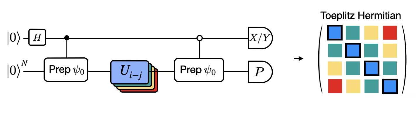
해밀토니안 $H$ 하에서 $|0\rangle^N$의 고유값인 $E_0$를 고전적으로 계산할 수 있다고 가정합니다. 이는 해밀토니안이 U(1) 대칭을 보존할 때 만족됩니다. 이것이 강한 가정처럼 보일 수 있지만, 해밀토니안의 작용에 영향을 받지 않는 진공 상태(이 경우 $|0\rangle^N$ 상태에 대응됨)가 존재한다고 가정하는 것이 안전한 경우가 많습니다. 예를 들어, 전자 수가 보존되는 안정적인 분자를 기술하는 화학 해밀토니안에서 이것이 사실입니다. 게이트 $\text{Prep} \; \psi$가 원하는 참조 상태 $\ket{psi} = \text{Prep} \; \psi \ket{0} = e^{-i H 0 dt} U_{\psi} \ket{0}$를 준비한다고 할 때, 예를 들어 화학에서 HF 상태를 준비하기 위해 $\text{Prep} \; \psi$는 단일 큐비트 NOT의 곱이 되므로, 제어형-$\text{Prep} \; \psi$는 단순히 CNOT의 곱이 됩니다. 그러면 위의 회로는 측정 전에 다음 상태를 구현합니다:

$$\begin{equation} \begin{split} \ket{0} \ket{0}^N\xrightarrow{H}&\frac{1}{\sqrt{2}} \left( \ket{0}\ket{0}^N+ \ket{1} \ket{0}^N \right)\\ \xrightarrow{\text{1-ctrl-init}}&\frac{1}{\sqrt{2}}\left(|0\rangle|0\rangle^N+|1\rangle|\psi\rangle\right)\\ \xrightarrow{U}&\frac{1}{\sqrt{2}}\left(e^{i\phi}\ket{0}\ket{0}^N+\ket{1} U\ket{\psi}\right)\\ \xrightarrow{\text{0-ctrl-init}}&\frac{1}{\sqrt{2}} \left( e^{i\phi}\ket{0} \ket{\psi} +\ket{1} U\ket{\psi} \right)\\ =&\frac{1}{2} \left( \ket{+}\left(e^{i\phi}\ket{\psi}+U\ket{\psi}\right) +\ket{-}\left(e^{i\phi}\ket{\psi}-U\ket{\psi}\right) \right)\\ =&\frac{1}{2} \left( \ket{+i}\left(e^{i\phi}\ket{\psi}-iU\ket{\psi}\right) +\ket{-i}\left(e^{i\phi}\ket{\psi}+iU\ket{\psi}\right) \right) \end{split} \end{equation}$$

여기서 세 번째 줄에서는 고전적으로 시뮬레이션 가능한 위상 이동 $U\ket{0}^N = e^{i\phi}\ket{0}^N$을 사용했습니다. 따라서 기댓값은 다음과 같이 구해집니다:

$$\begin{equation} \begin{split} \langle X\otimes P\rangle&=\frac{1}{4} \Big( \left(e^{-i\phi}\bra{\psi}+\bra{\psi}U^\dagger\right)P\left(e^{i\phi}\ket{\psi}+U\ket{\psi}\right) \\ &\qquad-\left(e^{-i\phi}\bra{\psi}-\bra{\psi}U^\dagger\right)P\left(e^{i\phi}\ket{\psi}-U\ket{\psi}\right) \Big)\\ &=\text{Re}\left[e^{-i\phi}\bra{\psi}PU\ket{\psi}\right], \end{split} \end{equation}$$ $$\begin{equation} \begin{split} \langle Y\otimes P\rangle&=\frac{1}{4} \Big( \left(e^{-i\phi}\bra{\psi}+i\bra{\psi}U^\dagger\right)P\left(e^{i\phi}\ket{\psi}-iU\ket{\psi}\right) \\ &\qquad-\left(e^{-i\phi}\bra{\psi}-i\bra{\psi}U^\dagger\right)P\left(e^{i\phi}\ket{\psi}+iU\ket{\psi}\right) \Big)\\ &=\text{Im}\left[e^{-i\phi}\bra{\psi}PU\ket{\psi}\right]. \end{split} \end{equation}$$

이러한 가정들을 통해 더 적은 수의 제어 연산으로 관심 있는 연산자의 기댓값을 쓸 수 있게 되었습니다. 실제로 제어형 시간 진화가 아닌 제어형 상태 준비 $\text{Prep} \; \psi$만 구현하면 됩니다. 위와 같이 계산을 재구성하면 결과 회로의 깊이를 크게 줄일 수 있습니다.

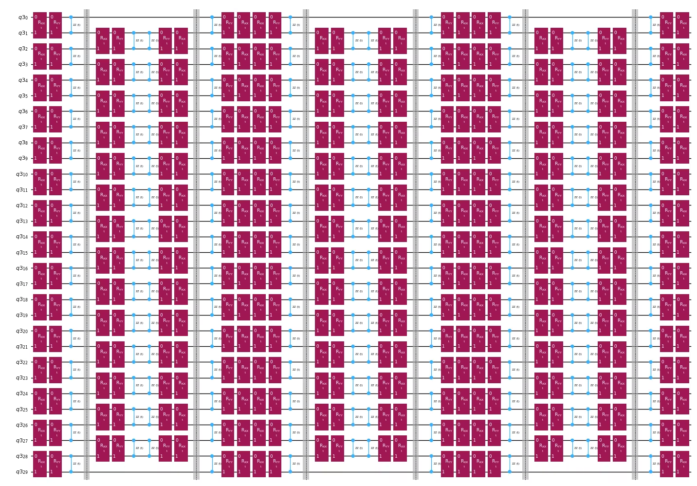
Trotter 분해로 시간 진화 연산자 분해

시간 진화 연산자를 정확하게 구현하는 대신 Trotter 분해를 사용하여 그것의 근사를 구현할 수 있습니다. 특정 차수의 Trotter 분해를 여러 번 반복하면 근사로 인해 도입되는 오차를 더욱 줄일 수 있습니다. 다음에서는 고려하는 해밀토니안의 상호작용 그래프(최근접 이웃 상호작용만)에 대해 가장 효율적인 방식으로 Trotter 구현을 직접 구축합니다. 실제로는 $e^{-i (XX + YY + ZZ) t}$의 근사 구현에 해당하는 매개변수화된 각도 $t$를 가진 Pauli 회전 $R_{xx}$, $R_{yy}$, $R_{zz}$를 삽입합니다. Pauli 회전의 정의와 구현하려는 시간 진화의 차이를 감안하여, $dt$의 시간 진화를 달성하려면 매개변수 $2*dt$를 사용해야 합니다. 또한, 홀수 번의 Trotter 단계 반복에 대해서는 연산 순서를 역전시키는데, 이는 기능적으로 동일하지만 인접한 연산을 단일 $SU(2)$ 유니타리로 합성할 수 있게 해줍니다. 이렇게 하면 일반적인 PauliEvolutionGate() 기능을 사용하여 얻는 것보다 훨씬 얕은 회로를 얻을 수 있습니다.

t = Parameter("t")

# Create instruction for rotation about XX+YY-ZZ:
Rxyz_circ = QuantumCircuit(2)
Rxyz_circ.rxx(t, 0, 1)
Rxyz_circ.ryy(t, 0, 1)
Rxyz_circ.rzz(t, 0, 1)
Rxyz_instr = Rxyz_circ.to_instruction(label="RXX+YY+ZZ")

interaction_list = [
    [[i, i + 1] for i in range(0, n_qubits - 1, 2)],
    [[i, i + 1] for i in range(1, n_qubits - 1, 2)],
]  # linear chain

qr = QuantumRegister(n_qubits)
trotter_step_circ = QuantumCircuit(qr)
for i, color in enumerate(interaction_list):
    for interaction in color:
        trotter_step_circ.append(Rxyz_instr, interaction)
    if i < len(interaction_list) - 1:
        trotter_step_circ.barrier()
reverse_trotter_step_circ = trotter_step_circ.reverse_ops()

qc_evol = QuantumCircuit(qr)
for step in range(num_trotter_steps):
    if step % 2 == 0:
        qc_evol = qc_evol.compose(trotter_step_circ)
    else:
        qc_evol = qc_evol.compose(reverse_trotter_step_circ)

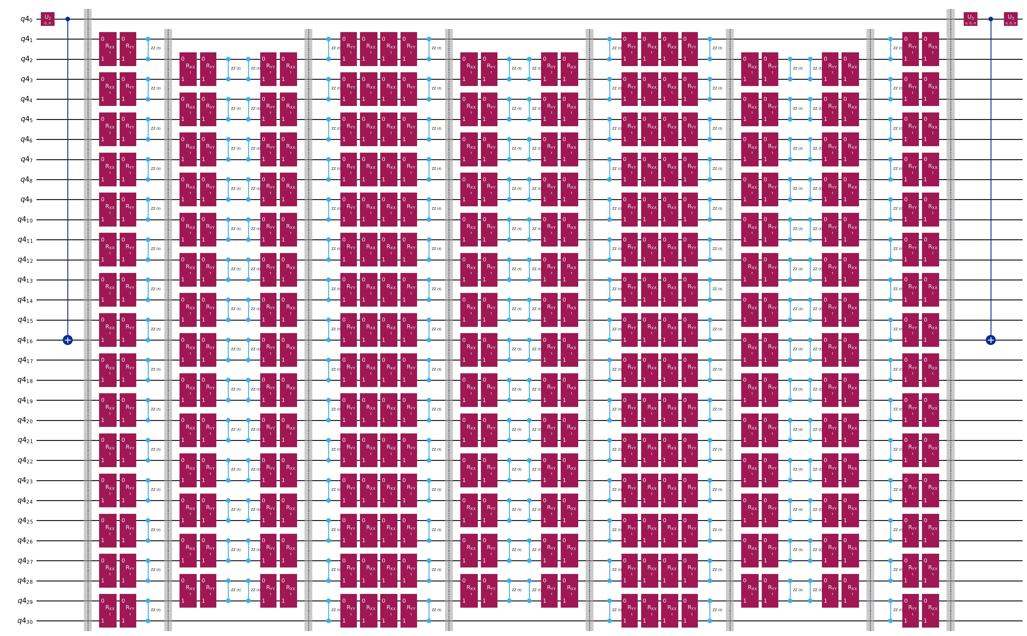
qc_evol.decompose().draw("mpl", fold=-1, scale=0.5)

상태 준비에 최적화된 회로 사용

control = 0
excitation = int(n_qubits / 2) + 1
controlled_state_prep = QuantumCircuit(n_qubits + 1)
controlled_state_prep.cx(control, excitation)
controlled_state_prep.draw("mpl", fold=-1, scale=0.5)

하다마르 테스트를 통한 $\tilde{S}$ 및 $\tilde{H}$ 행렬 요소 계산을 위한 템플릿 회로

하다마르 테스트에서 사용되는 회로 간의 유일한 차이는 시간 진화 연산자의 위상과 측정되는 관측량입니다. 따라서 시간 진화 연산자에 의존하는 게이트에 대한 플레이스홀더를 포함하여 하다마르 테스트의 일반 회로를 나타내는 템플릿 회로를 준비할 수 있습니다.

# Parameters for the template circuits
parameters = []
for idx in range(1, krylov_dim):
    parameters.append(2 * dt_circ * (idx))

# Create modified hadamard test circuit
qr = QuantumRegister(n_qubits + 1)
qc = QuantumCircuit(qr)
qc.h(0)
qc.compose(controlled_state_prep, list(range(n_qubits + 1)), inplace=True)
qc.barrier()
qc.compose(qc_evol, list(range(1, n_qubits + 1)), inplace=True)
qc.barrier()
qc.x(0)
qc.compose(
    controlled_state_prep.inverse(), list(range(n_qubits + 1)), inplace=True
)
qc.x(0)

qc.decompose().draw("mpl", fold=-1)

print(
    "The optimized circuit has 2Q gates depth: ",
    qc.decompose().decompose().depth(lambda x: x[0].num_qubits == 2),
)

The optimized circuit has 2Q gates depth:  74

Trotter 근사와 비제어 유니타리를 조합하여 하다마르 테스트의 깊이를 상당히 줄였습니다.

Step 3: Qiskit 프리미티브를 사용한 실행

Backend를 인스턴스화하고 런타임 매개변수를 설정합니다.

service = QiskitRuntimeService()
backend = service.least_busy(operational=True, simulator=False)
if (
    "if_else" not in backend.target.operation_names
):  # Needed as "op_name" could be "if_else"
    backend.target.add_instruction(IfElseOp, name="if_else")
print(backend.name)

QPU로 트랜스파일하기

먼저, 커플링 맵에서 성능이 "좋은" 큐비트 부분 집합을 선택하겠습니다("좋다"는 것은 다소 임의적인 기준으로, 주로 성능이 매우 낮은 큐비트를 피하려는 것입니다). 그런 다음 트랜스파일을 위한 새 타겟을 생성합니다.

target = backend.target
cmap = target.build_coupling_map(filter_idle_qubits=True)
cmap_list = list(cmap.get_edges())

cust_cmap_list = copy.deepcopy(cmap_list)
for q in range(target.num_qubits):
    meas_err = target["measure"][(q,)].error
    t2 = target.qubit_properties[q].t2 * 1e6
    if meas_err > 0.02 or t2 < 100:
        for q_pair in cmap_list:
            if q in q_pair:
                try:
                    cust_cmap_list.remove(q_pair)
                except:
                    continue

for q in cmap_list:
    op_name = list(target.operation_names_for_qargs(q))[0]
    twoq_gate_err = target[f"{op_name}"][q].error
    if twoq_gate_err > 0.005:
        for q_pair in cmap_list:
            if q == q_pair:
                try:
                    cust_cmap_list.remove(q)
                except:
                    continue

cust_cmap = CouplingMap(cust_cmap_list)
cust_target = Target.from_configuration(
    basis_gates=backend.configuration().basis_gates,
    coupling_map=cust_cmap,
)

그런 다음 가상 Circuit을 이 새 타겟의 최적 물리 레이아웃으로 트랜스파일합니다.

basis_gates = list(target.operation_names)
pm = generate_preset_pass_manager(
    optimization_level=3,
    target=cust_target,
    basis_gates=basis_gates,
)

qc_trans = pm.run(qc)

print("depth", qc_trans.depth(lambda x: x[0].num_qubits == 2))
print("num 2q ops", qc_trans.count_ops())
print(
    "physical qubits",
    sorted(
        [
            idx
            for idx, qb in qc_trans.layout.initial_layout.get_physical_bits().items()
            if qb._register.name != "ancilla"
        ]
    ),
)

depth 52
num 2q ops OrderedDict([('rz', 2058), ('sx', 1703), ('cz', 728), ('x', 84), ('barrier', 8)])
physical qubits [91, 92, 93, 94, 95, 98, 99, 108, 109, 110, 111, 113, 114, 115, 119, 127, 132, 133, 134, 135, 137, 139, 147, 148, 149, 150, 151, 152, 153, 154, 155]

Estimator로 실행할 PUB 생성하기

# Define observables to measure for S
observable_S_real = "I" * (n_qubits) + "X"
observable_S_imag = "I" * (n_qubits) + "Y"

observable_op_real = SparsePauliOp(
    observable_S_real
)  # define a sparse pauli operator for the observable
observable_op_imag = SparsePauliOp(observable_S_imag)

layout = qc_trans.layout  # get layout of transpiled circuit
observable_op_real = observable_op_real.apply_layout(
    layout
)  # apply physical layout to the observable
observable_op_imag = observable_op_imag.apply_layout(layout)
observable_S_real = (
    observable_op_real.paulis.to_labels()
)  # get the label of the physical observable
observable_S_imag = observable_op_imag.paulis.to_labels()

observables_S = [[observable_S_real], [observable_S_imag]]

# Define observables to measure for H
# Hamiltonian terms to measure
observable_list = []
for pauli, coeff in zip(H_op.paulis, H_op.coeffs):
    # print(pauli)
    observable_H_real = pauli[::-1].to_label() + "X"
    observable_H_imag = pauli[::-1].to_label() + "Y"
    observable_list.append([observable_H_real])
    observable_list.append([observable_H_imag])

layout = qc_trans.layout

observable_trans_list = []
for observable in observable_list:
    observable_op = SparsePauliOp(observable)
    observable_op = observable_op.apply_layout(layout)
    observable_trans_list.append([observable_op.paulis.to_labels()])

observables_H = observable_trans_list

# Define a sweep over parameter values
params = np.vstack(parameters).T

# Estimate the expectation value for all combinations of
# observables and parameter values, where the pub result will have
# shape (# observables, # parameter values).
pub = (qc_trans, observables_S + observables_H, params)

Circuit 실행하기

$t=0$에 대한 Circuit은 고전적으로 계산할 수 있습니다.

qc_cliff = qc.assign_parameters({t: 0})

# Get expectation values from experiment
S_expval_real = StabilizerState(qc_cliff).expectation_value(
    Pauli("I" * (n_qubits) + "X")
)
S_expval_imag = StabilizerState(qc_cliff).expectation_value(
    Pauli("I" * (n_qubits) + "Y")
)

# Get expectation values
S_expval = S_expval_real + 1j * S_expval_imag

H_expval = 0
for obs_idx, (pauli, coeff) in enumerate(zip(H_op.paulis, H_op.coeffs)):
    # Get expectation values from experiment
    expval_real = StabilizerState(qc_cliff).expectation_value(
        Pauli(pauli[::-1].to_label() + "X")
    )
    expval_imag = StabilizerState(qc_cliff).expectation_value(
        Pauli(pauli[::-1].to_label() + "Y")
    )
    expval = expval_real + 1j * expval_imag

    # Fill-in matrix elements
    H_expval += coeff * expval

print(H_expval)

(25+0j)

Estimator를 사용하여 $S$와 $\tilde{H}$에 대한 Circuit을 실행합니다.

# Experiment options
num_randomizations = 300
num_randomizations_learning = 30
shots_per_randomization = 100
noise_factors = [1, 1.2, 1.4]
learning_pair_depths = [0, 4, 24, 48]

experimental_opts = {}
experimental_opts["resilience"] = {
    "measure_mitigation": True,
    "measure_noise_learning": {
        "num_randomizations": num_randomizations_learning,
        "shots_per_randomization": shots_per_randomization,
    },
    "zne_mitigation": True,
    "zne": {"noise_factors": noise_factors},
    "layer_noise_learning": {
        "max_layers_to_learn": 10,
        "layer_pair_depths": learning_pair_depths,
        "shots_per_randomization": shots_per_randomization,
        "num_randomizations": num_randomizations_learning,
    },
    "zne": {
        "amplifier": "pea",
        "extrapolated_noise_factors": [0] + noise_factors,
    },
}
experimental_opts["twirling"] = {
    "num_randomizations": num_randomizations,
    "shots_per_randomization": shots_per_randomization,
    "strategy": "all",
}

estimator = Estimator(mode=backend, options=experimental_opts)

job = estimator.run([pub])

4단계: 후처리 및 원하는 고전적 형식으로 결과 반환

results = job.result()[0]

유효 해밀토니안 및 겹침 행렬 계산

먼저, 비제어 시간 진화 동안 $\vert 0 \rangle$ 상태가 축적한 위상을 계산합니다.

prefactors = [
    np.exp(-1j * sum([c for p, c in H_op.to_list() if "Z" in p]) * i * dt)
    for i in range(1, krylov_dim)
]

회로 실행 결과를 얻은 후에는 데이터를 후처리하여 $S$의 행렬 원소를 계산할 수 있습니다.

# Assemble S, the overlap matrix of dimension D:
S_first_row = np.zeros(krylov_dim, dtype=complex)
S_first_row[0] = 1 + 0j

# Add in ancilla-only measurements:
for i in range(krylov_dim - 1):
    # Get expectation values from experiment
    expval_real = results.data.evs[0][0][
        i
    ]  # automatic extrapolated evs if ZNE is used
    expval_imag = results.data.evs[1][0][
        i
    ]  # automatic extrapolated evs if ZNE is used

    # Get expectation values
    expval = expval_real + 1j * expval_imag
    S_first_row[i + 1] += prefactors[i] * expval

S_first_row_list = S_first_row.tolist()  # for saving purposes

S_circ = np.zeros((krylov_dim, krylov_dim), dtype=complex)

# Distribute entries from first row across matrix:
for i, j in it.product(range(krylov_dim), repeat=2):
    if i >= j:
        S_circ[j, i] = S_first_row[i - j]
    else:
        S_circ[j, i] = np.conj(S_first_row[j - i])

Matrix(S_circ)

$$\displaystyle \left[\begin{matrix}1.0 & -0.723052998582984 - 0.345085413575966 i & 0.467051960502366 + 0.516197865254034 i & -0.180546747798251 - 0.492624093654174 i & 0.0012070853532697 + 0.312052218182462 i\\-0.723052998582984 + 0.345085413575966 i & 1.0 & -0.723052998582984 - 0.345085413575966 i & 0.467051960502366 + 0.516197865254034 i & -0.180546747798251 - 0.492624093654174 i\\0.467051960502366 - 0.516197865254034 i & -0.723052998582984 + 0.345085413575966 i & 1.0 & -0.723052998582984 - 0.345085413575966 i & 0.467051960502366 + 0.516197865254034 i\\-0.180546747798251 + 0.492624093654174 i & 0.467051960502366 - 0.516197865254034 i & -0.723052998582984 + 0.345085413575966 i & 1.0 & -0.723052998582984 - 0.345085413575966 i\\0.0012070853532697 - 0.312052218182462 i & -0.180546747798251 + 0.492624093654174 i & 0.467051960502366 - 0.516197865254034 i & -0.723052998582984 + 0.345085413575966 i & 1.0\end{matrix}\right]$$

그리고 $\tilde{H}$의 행렬 원소를 계산합니다.

# Assemble S, the overlap matrix of dimension D:
H_first_row = np.zeros(krylov_dim, dtype=complex)
H_first_row[0] = H_expval

for obs_idx, (pauli, coeff) in enumerate(zip(H_op.paulis, H_op.coeffs)):
    # Add in ancilla-only measurements:
    for i in range(krylov_dim - 1):
        # Get expectation values from experiment
        expval_real = results.data.evs[2 + 2 * obs_idx][0][
            i
        ]  # automatic extrapolated evs if ZNE is used
        expval_imag = results.data.evs[2 + 2 * obs_idx + 1][0][
            i
        ]  # automatic extrapolated evs if ZNE is used

        # Get expectation values
        expval = expval_real + 1j * expval_imag
        H_first_row[i + 1] += prefactors[i] * coeff * expval

H_first_row_list = H_first_row.tolist()

H_eff_circ = np.zeros((krylov_dim, krylov_dim), dtype=complex)

# Distribute entries from first row across matrix:
for i, j in it.product(range(krylov_dim), repeat=2):
    if i >= j:
        H_eff_circ[j, i] = H_first_row[i - j]
    else:
        H_eff_circ[j, i] = np.conj(H_first_row[j - i])

Matrix(H_eff_circ)

$$\displaystyle \left[\begin{matrix}25.0 & -14.2437089383409 - 6.50486277982165 i & 10.2857217968584 + 9.0431912203186 i & -5.15587257589417 - 8.88280836036843 i & 1.98818301405581 + 5.8897614762563 i\\-14.2437089383409 + 6.50486277982165 i & 25.0 & -14.2437089383409 - 6.50486277982165 i & 10.2857217968584 + 9.0431912203186 i & -5.15587257589417 - 8.88280836036843 i\\10.2857217968584 - 9.0431912203186 i & -14.2437089383409 + 6.50486277982165 i & 25.0 & -14.2437089383409 - 6.50486277982165 i & 10.2857217968584 + 9.0431912203186 i\\-5.15587257589417 + 8.88280836036843 i & 10.2857217968584 - 9.0431912203186 i & -14.2437089383409 + 6.50486277982165 i & 25.0 & -14.2437089383409 - 6.50486277982165 i\\1.98818301405581 - 5.8897614762563 i & -5.15587257589417 + 8.88280836036843 i & 10.2857217968584 - 9.0431912203186 i & -14.2437089383409 + 6.50486277982165 i & 25.0\end{matrix}\right]$$

마지막으로, $\tilde{H}$에 대한 일반화 고유값 문제를 풀 수 있습니다.

$\tilde{H} \vec{c} = c S \vec{c}$

그리고 바닥 상태 에너지 $c_{min}$의 추정값을 얻습니다.

gnd_en_circ_est_list = []
for d in range(1, krylov_dim + 1):
    # Solve generalized eigenvalue problem for different size of the Krylov space
    gnd_en_circ_est = solve_regularized_gen_eig(
        H_eff_circ[:d, :d], S_circ[:d, :d], threshold=9e-1
    )
    gnd_en_circ_est_list.append(gnd_en_circ_est)
    print("The estimated ground state energy is: ", gnd_en_circ_est)

The estimated ground state energy is:  25.0
The estimated ground state energy is:  22.572154819954875
The estimated ground state energy is:  21.691509219286587
The estimated ground state energy is:  21.23882298756386
The estimated ground state energy is:  20.965499325470294

단일 입자 부문의 경우, 이 해밀토니안 부문의 바닥 상태를 고전적으로 효율적으로 계산할 수 있습니다.

gs_en = single_particle_gs(H_op, n_qubits)

n_sys_qubits 30
n_exc 1 , subspace dimension 31
single particle ground state energy:  21.021912418526906

plt.plot(
    range(1, krylov_dim + 1),
    gnd_en_circ_est_list,
    color="blue",
    linestyle="-.",
    label="KQD estimate",
)
plt.plot(
    range(1, krylov_dim + 1),
    [gs_en] * krylov_dim,
    color="red",
    linestyle="-",
    label="exact",
)
plt.xticks(range(1, krylov_dim + 1), range(1, krylov_dim + 1))
plt.legend()
plt.xlabel("Krylov space dimension")
plt.ylabel("Energy")
plt.title(
    "Estimating Ground state energy with Krylov Quantum Diagonalization"
)
plt.show()

부록: 실수 시간 진화를 통한 Krylov 부분 공간

유니터리 Krylov 공간은 다음과 같이 정의됩니다.

$$\mathcal{K}_U(H, |\psi\rangle) = \text{span}\left\{ |\psi\rangle, e^{-iH\,dt} |\psi\rangle, \dots, e^{-irH\,dt} |\psi\rangle \right\}$$

이때 $dt$는 나중에 결정할 시간 간격입니다. 잠시 $r$이 짝수라고 가정하면, $d=r/2$로 정의할 수 있습니다. 해밀토니안을 위의 Krylov 공간에 투영할 때, 아래의 Krylov 공간과 구별할 수 없다는 점에 주목하세요.

$$\mathcal{K}_U(H, |\psi\rangle) = \text{span}\left\{ e^{i\,d\,H\,dt}|\psi\rangle, e^{i(d-1)H\,dt} |\psi\rangle, \dots, e^{-i(d-1)H\,dt} |\psi\rangle, e^{-i\,d\,H\,dt} |\psi\rangle \right\},$$

즉, 모든 시간 진화가 $d$ 시간 간격만큼 뒤로 이동된 경우입니다. 구별할 수 없는 이유는 행렬 원소

$$\tilde{H}_{j,k} = \langle\psi|e^{i\,j\,H\,dt}He^{-i\,k\,H\,dt}|\psi\rangle=\langle\psi|He^{i(j-k)H\,dt}|\psi\rangle$$

가 시간 진화가 해밀토니안과 교환 가능하기 때문에, 진화 시간의 전체적인 이동에 대해 불변이기 때문입니다. $r$이 홀수인 경우에는 $r-1$에 대한 분석을 사용할 수 있습니다.

이 Krylov 공간 어딘가에 저에너지 상태가 반드시 존재함을 보이고자 합니다. 이를 위해 [3]의 정리 3.1에서 도출된 다음 결과를 사용합니다.

주장 1: 해밀토니안의 스펙트럼 범위(바닥 상태 에너지와 최대 에너지 사이)에 있는 에너지 $E$에 대해 함수 $f$가 존재하여...

1. $f(E_0)=1$
2. $E_0$으로부터 $\ge\delta$ 떨어진 모든 $E$ 값에 대해 $|f(E)|\le2\left(1 + \delta\right)^{-d}$ (즉, 지수적으로 억제됨)
3. $f(E)$는 $j=-d,-d+1,...,d-1,d$에 대한 $e^{ijE\,dt}$의 선형 결합

아래에 증명을 제공하지만, 완전하고 엄밀한 논증을 이해하고 싶지 않다면 건너뛰어도 됩니다. 지금은 위 주장의 함의에 집중하겠습니다. 위의 성질 3에 의해, 위에서 이동된 Krylov 공간에는 상태 $f(H)|\psi\rangle$이 포함된다는 것을 알 수 있습니다. 이것이 저에너지 상태입니다. 이를 확인하기 위해 에너지 고유 기저로 $|\psi\rangle$을 전개하면:

$$|\psi\rangle = \sum_{k=0}^{N}\gamma_k|E_k\rangle,$$

여기서 $|E_k\rangle$은 $k$번째 에너지 고유 상태이고 $\gamma_k$는 초기 상태 $|\psi\rangle$에서의 진폭입니다. 이를 이용하면 $f(H)|\psi\rangle$은

$$f(H)|\psi\rangle = \sum_{k=0}^{N}\gamma_kf(E_k)|E_k\rangle,$$

$H$가 고유 상태 $|E_k\rangle$에 작용할 때 $E_k$로 대체할 수 있다는 사실을 이용한 것입니다. 따라서 이 상태의 에너지 오차는

$$\text{energy error} = \frac{\langle\psi|f(H)(H-E_0)f(H)|\psi\rangle}{\langle\psi|f(H)^2|\psi\rangle}$$ $$= \frac{\sum_{k=0}^{N}|\gamma_k|^2f(E_k)^2(E_k-E_0)}{\sum_{k=0}^{N}|\gamma_k|^2f(E_k)^2}.$$

이해하기 쉬운 상한으로 변환하기 위해, 분자의 합을 $E_k-E_0\le\delta$인 항과 $E_k-E_0>\delta$인 항으로 분리합니다.

$$\text{energy error} = \frac{\sum_{E_k\le E_0+\delta}|\gamma_k|^2f(E_k)^2(E_k-E_0)}{\sum_{k=0}^{N}|\gamma_k|^2f(E_k)^2} + \frac{\sum_{E_k> E_0+\delta}|\gamma_k|^2f(E_k)^2(E_k-E_0)}{\sum_{k=0}^{N}|\gamma_k|^2f(E_k)^2}.$$

첫 번째 항은 $\delta$로 상한을 구할 수 있습니다.

$$\frac{\sum_{E_k\le E_0+\delta}|\gamma_k|^2f(E_k)^2(E_k-E_0)}{\sum_{k=0}^{N}|\gamma_k|^2f(E_k)^2} < \frac{\delta\sum_{E_k\le E_0+\delta}|\gamma_k|^2f(E_k)^2}{\sum_{k=0}^{N}|\gamma_k|^2f(E_k)^2} \le \delta,$$

첫 번째 단계는 합산의 모든 $E_k$에 대해 $E_k-E_0\le\delta$이기 때문이고, 두 번째 단계는 분자의 합이 분모의 합의 부분 집합이기 때문입니다. 두 번째 항의 경우, $f(E_0)^2=1$이므로 분모를 $|\gamma_0|^2$로 하한 처리합니다. 모두 합치면,

$$\text{energy error} \le \delta + \frac{1}{|\gamma_0|^2}\sum_{E_k>E_0+\delta}|\gamma_k|^2f(E_k)^2(E_k-E_0).$$

나머지를 단순화하기 위해, 이 모든 $E_k$에 대해 $f$의 정의로부터 $f(E_k)^2 \le 4\left(1 + \delta\right)^{-2d}$임을 알 수 있습니다. 또한 $E_k-E_0<2\|H\|$로 상한 처리하고 $\sum_{E_k>E_0+\delta}|\gamma_k|^2<1$로 상한 처리하면

$$\text{energy error} \le \delta + \frac{8}{|\gamma_0|^2}\|H\|\left(1 + \delta\right)^{-2d}.$$

이는 임의의 $\delta>0$에 대해 성립하므로, $\delta$를 목표 오차와 같게 설정하면 위의 오차 상한은 Krylov 차원 $2d=r$에 따라 지수적으로 수렴합니다. 또한 $\delta<E_1-E_0$이면 위의 상한에서 $\delta$ 항이 완전히 사라집니다.

논증을 완성하기 위해, 위는 Krylov 공간에서 가장 낮은 에너지 상태의 에너지 오차가 아니라 특정 상태 $f(H)|\psi\rangle$의 에너지 오차임을 먼저 주목합니다. 그러나 (Rayleigh-Ritz) 변분 원리에 의해, Krylov 공간에서 가장 낮은 에너지 상태의 에너지 오차는 Krylov 공간의 어떤 상태의 에너지 오차로도 상한을 구할 수 있으므로, 위는 가장 낮은 에너지 상태, 즉 Krylov 양자 대각화 알고리즘의 출력의 에너지 오차에 대한 상한이기도 합니다.

위와 유사한 분석을 통해 노이즈와 노트북에서 논의된 임계값 처리 절차까지 추가로 고려할 수 있습니다. 이 분석은 [2] 및 [4]를 참조하세요.

부록: 주장 1의 증명

다음은 주로 [3] 정리 3.1에서 도출된 것입니다. $0 < a < b$ 이고 $\Pi^*_d$를 차수가 최대 $d$인 잔류 다항식(0에서 값이 1인 다항식)의 공간이라 하면,

$$\beta(a, b, d) = \min_{p \in \Pi^*_d} \max_{x \in [a, b]} |p(x)| \quad$$

의 해는

$$p^*(x) = \frac{T_d\left(\frac{b + a - 2x}{b - a}\right)}{T_d\left(\frac{b + a}{b - a}\right)}, \quad$$

이고 대응하는 최솟값은

$$\beta(a, b, d) = T_d^{-1}\left(\frac{b + a}{b - a}\right).$$

이것을 복소 지수 함수로 자연스럽게 표현할 수 있는 함수로 변환하고자 합니다. 복소 지수 함수는 양자 Krylov 공간을 생성하는 실수 시간 진화이기 때문입니다. 이를 위해 해밀토니안의 스펙트럼 범위 내 에너지를 $[0,1]$ 범위의 숫자로 변환하는 다음 변환을 도입하는 것이 편리합니다.

$$g(E) = \frac{1-\cos\big((E-E_0)dt\big)}{2},$$

여기서 $dt$는 $-\pi < E_0dt < E_\text{max}dt < \pi$인 시간 간격입니다. $g(E_0)=0$이고 $E$가 $E_0$에서 멀어질수록 $g(E)$가 커집니다.

이제 매개변수 a, b, d를 $a = g(E_0 + \delta)$, $b = 1$, d = int(r/2)로 설정한 다항식 $p^*(x)$를 사용하여 다음 함수를 정의합니다.

$$f(E) = p^* \left( g(E) \right) = \frac{T_d\left(1 + 2\frac{\cos\big((E-E_0)dt\big) - \cos\big(\delta\,dt\big)}{1 +\cos\big(\delta\,dt\big)}\right)}{T_d\left(1 + 2\frac{1-\cos\big(\delta\,dt\big)}{1 + \cos\big(\delta\,dt\big)}\right)}$$

여기서 $E_0$은 바닥 상태 에너지입니다. $\cos(x)=\frac{e^{ix}+e^{-ix}}{2}$를 대입하면 $f(E)$는 차수 $d$의 삼각 다항식, 즉 $j=-d,-d+1,...,d-1,d$에 대한 $e^{ijE\,dt}$의 선형 결합임을 알 수 있습니다. 더불어, 위의 $p^*(x)$의 정의로부터 $f(E_0)=p(0)=1$이고, $\vert E-E_0 \vert > \delta$인 스펙트럼 범위 내의 임의의 $E$에 대해

$$|f(E)| \le \beta(a, b, d) = T_d^{-1}\left(1 + 2\frac{1-\cos\big(\delta\,dt\big)}{1 + \cos\big(\delta\,dt\big)}\right)$$ $$\leq 2\left(1 + \delta\right)^{-d} = 2\left(1 + \delta\right)^{-\lfloor k/2\rfloor}.$$

참고 문헌

[1] N. Yoshioka, M. Amico, W. Kirby et al. "Diagonalization of large many-body Hamiltonians on a quantum processor". arXiv:2407.14431

[2] Ethan N. Epperly, Lin Lin, and Yuji Nakatsukasa. "A theory of quantum subspace diagonalization". SIAM Journal on Matrix Analysis and Applications 43, 1263–1290 (2022).

[3] Å. Björck. "Numerical methods in matrix computations". Texts in Applied Mathematics. Springer International Publishing. (2014).

[4] William Kirby. "Analysis of quantum Krylov algorithms with errors". Quantum 8, 1457 (2024).

튜토리얼 설문

이 튜토리얼에 대한 피드백을 제공하기 위해 짧은 설문에 참여해 주세요. 여러분의 의견은 콘텐츠 개선과 사용자 경험 향상에 도움이 됩니다.

설문 링크

Note: This survey is provided by IBM Quantum and relates to the original English content. To give feedback on doQumentation's website, translations, or code execution, please open a GitHub issue.