양자 근사 최적화 알고리즘

사용 시간 예상: Heron r3 프로세서 기준 22분 (참고: 이는 예상치이며 실제 실행 시간은 다를 수 있습니다.)

학습 성과

이 튜토리얼을 완료하면 다음 정보를 이해할 수 있게 됩니다:

• 고전적 조합 최적화 문제(max-cut)를 양자 Hamiltonian으로 매핑하는 방법
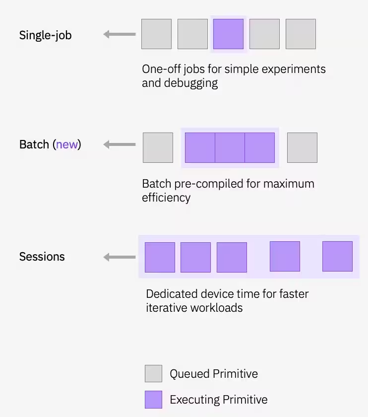
• Qiskit Runtime Session을 사용하여 양자 근사 최적화 알고리즘(QAOA)을 구현하고 실행하는 방법
• 작은 시뮬레이터 예제에서 유틸리티 규모의 하드웨어 실행으로 QAOA 워크플로를 확장하는 방법

사전 준비 사항

다음 주제에 익숙해지는 것을 권장합니다:

• 양자 Circuit의 기초
• 변분 알고리즘
• QAOA 심화 — QAOA 알고리즘에 대한 포괄적인 설명과 유틸리티 규모에서의 적용

배경

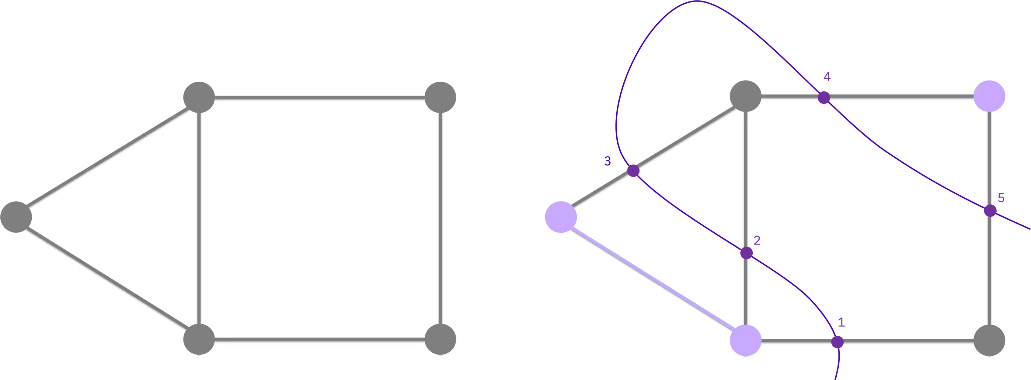
**양자 근사 최적화 알고리즘(Quantum Approximate Optimization Algorithm, QAOA)**은 조합 최적화 문제를 해결하기 위한 하이브리드 양자-고전 반복 방법입니다. 이 튜토리얼에서는 QAOA를 사용하여 최대 컷(maximum-cut, max-cut) 문제 — 클러스터링, 네트워크 과학, 통계 물리학 등에 응용되는 NP-hard 최적화 문제 — 를 해결합니다. 엣지로 연결된 노드로 구성된 그래프가 주어졌을 때, 목표는 분할을 가로지르는 엣지의 수가 최대화되도록 노드를 두 집합으로 나누는 것입니다.

고전적 최적화에서 양자 Circuit으로

Max-cut은 고전적인 이진 최적화 문제로 표현될 수 있습니다. 각 노드에는 어느 집합에 속하는지를 나타내는 이진 변수 $x_i \in \{0, 1\}$가 할당됩니다. 목표는 양 끝점이 서로 다른 집합에 속하는 엣지의 수를 최대화하는 것입니다:

$$\max_{x \in \{0,1\}^n} \sum_{(i,j)} x_i + x_j - 2x_ix_j.$$

이는 동등하게 $\min_x\, x^T Q x$ 형태의 이차 비제약 이진 최적화(Quadratic Unconstrained Binary Optimization, QUBO) 문제입니다. 표준적인 변수 치환($x_i \to (1 - Z_i)/2$)을 통해 QUBO는 기저 상태가 최적해를 인코딩하는 비용 Hamiltonian으로 다시 쓸 수 있습니다. 일반적으로 이 Hamiltonian은 이차 항과 선형 항을 모두 가집니다:

$$H_C = \sum_{ij} Q_{ij} \, Z_i Z_j + \sum_i b_i \, Z_i.$$

여기서 고려하는 비가중 max-cut 문제의 경우 선형 계수가 소멸하고($b_i = 0$) 각 엣지에 대해 $Q_{ij} = 1$이므로, 아래 코드에서 구축할 더 간단한 형태 $H_C = \sum_{(i,j) \in E} Z_i Z_j$가 남습니다. 위의 더 일반적인 형태는 이 워크플로를 가중 그래프나 기타 QUBO로 표현 가능한 문제에 적용하려고 할 때 필요한 형태입니다.

QAOA의 작동 방식

QAOA는 초기 중첩 상태 $H^{\otimes n}|0\rangle$에 두 연산자의 교대 레이어를 적용하여 후보 해를 준비합니다: 비용 연산자 $e^{-i\gamma_k H_C}$와 믹서 연산자 $e^{-i\beta_k H_m}$입니다. 각도 $\gamma_k$와 $\beta_k$는 고전적 피드백 루프에서 최적화됩니다; 양자 컴퓨터는 비용 함수를 평가하고, 고전적 최적화기는 수렴할 때까지 파라미터를 업데이트합니다. 이 반복 루프는 Qiskit Runtime Session 내에서 실행되며, 이는 반복 전반에 걸쳐 양자 장치를 예약 상태로 유지하여 지연 시간을 낮춥니다.

전체 QUBO-Hamiltonian 유도를 포함한 QAOA 이론에 대한 더 깊은 설명은 QAOA 코스 모듈을 참고하세요.

이 튜토리얼에서는 먼저 작은 5-노드 그래프에서 max-cut을 해결한 다음, 동일한 워크플로를 실제 하드웨어의 100-노드 유틸리티 규모 문제로 확장합니다. 플랜 접근에 대한 참고: 이 튜토리얼은 Qiskit Runtime Session을 사용하며, 이는 Premium Plan에서만 사용할 수 있습니다. Open Plan을 사용하는 경우 작성된 그대로 이 튜토리얼을 실행할 수 없습니다; 대신 Session을 job 모드로 교체해야 합니다(즉, 최적화 루프를 with Session(...)으로 감싸는 대신 각 반복을 독립적인 작업으로 제출). 워크플로는 여전히 실행되지만, 예약된 장치를 재사용하는 대신 각 반복이 전체 대기열 지연 시간을 겪게 됩니다. 자세한 내용은 사용 가능한 플랜 개요를 참고하세요.

요구 사항

이 튜토리얼을 시작하기 전에 다음이 설치되어 있는지 확인하세요:

• Qiskit SDK v2.0 이상 (시각화 지원 포함)
• Qiskit Runtime v0.22 이상 (pip install qiskit-ibm-runtime)

또한 IBM Quantum® Platform의 인스턴스에 접근 권한이 필요합니다.

설정

# Added by doQumentation — required packages for this notebook
!pip install -q matplotlib numpy qiskit qiskit-ibm-runtime rustworkx scipy

import matplotlib.pyplot as plt
import rustworkx as rx
from rustworkx.visualization import mpl_draw as draw_graph
import numpy as np
from scipy.optimize import minimize
from collections import defaultdict
from typing import Sequence

from qiskit.quantum_info import SparsePauliOp
from qiskit.circuit.library import QAOAAnsatz
from qiskit.transpiler.preset_passmanagers import generate_preset_pass_manager

from qiskit_ibm_runtime import QiskitRuntimeService
from qiskit_ibm_runtime import Session, EstimatorV2 as Estimator
from qiskit_ibm_runtime import SamplerV2 as Sampler

소규모 예제

이 섹션에서는 작은 5-노드 max-cut 인스턴스에서 QAOA 워크플로의 각 단계를 살펴봅니다. "소규모"라는 라벨에도 불구하고, 이 예제는 여전히 실제 IBM Quantum 하드웨어에서 실행됩니다 — 코드는 127개 이상의 Qubit을 가진 Backend를 선택하고 거기서 Circuit을 실행합니다. $n=5$개의 노드를 가진 그래프를 생성하여 문제를 초기화합니다.

n_small = 5

graph = rx.PyGraph()
graph.add_nodes_from(np.arange(0, n_small, 1))
edge_list = [
    (0, 1, 1.0),
    (0, 2, 1.0),
    (0, 4, 1.0),
    (1, 2, 1.0),
    (2, 3, 1.0),
    (3, 4, 1.0),
]
graph.add_edges_from(edge_list)
draw_graph(graph, node_size=600, with_labels=True)

Step 1: 고전적 입력을 양자 문제로 매핑하기

고전적 그래프를 양자 Circuit과 연산자로 매핑합니다. 배경에서 설명한 대로, 비가중 max-cut의 경우 비용 Hamiltonian은 $H_C = \sum_{(i,j) \in E} Z_i Z_j$로 축소되며, QAOA는 매개변수화된 ansatz Circuit을 사용하여 $H_C$의 후보 기저 상태를 준비합니다.

비용 Hamiltonian 구축

그래프 엣지를 Pauli $Z_iZ_j$ 항으로 변환하여 $H_C$를 구축합니다(배경에서 유도 참고).

def build_max_cut_paulis(
    graph: rx.PyGraph,
) -> list[tuple[str, list[int], float]]:
    """Convert graph edges to a list of ZZ Pauli terms.

    The returned list is in the sparse format expected by
    ``SparsePauliOp.from_sparse_list``: each element is
    ``(pauli_string, qubit_indices, coefficient)``.
    """
    pauli_list = []
    for edge in list(graph.edge_list()):
        weight = graph.get_edge_data(edge[0], edge[1])
        pauli_list.append(("ZZ", [edge[0], edge[1]], weight))
    return pauli_list

max_cut_paulis = build_max_cut_paulis(graph)
cost_hamiltonian = SparsePauliOp.from_sparse_list(max_cut_paulis, n_small)
print("Cost Function Hamiltonian:", cost_hamiltonian)

Cost Function Hamiltonian: SparsePauliOp(['IIIZZ', 'IIZIZ', 'ZIIIZ', 'IIZZI', 'IZZII', 'ZZIII'],
              coeffs=[1.+0.j, 1.+0.j, 1.+0.j, 1.+0.j, 1.+0.j, 1.+0.j])

QAOA ansatz Circuit 구축

QAOAAnsatz를 사용하여 비용 Hamiltonian으로부터 매개변수화된 QAOA Circuit을 구축합니다. 여기서는 reps=2(두 개의 QAOA 레이어, 네 개의 파라미터: $\beta_0, \beta_1, \gamma_0, \gamma_1$)를 사용합니다.

circuit = QAOAAnsatz(cost_operator=cost_hamiltonian, reps=2)
circuit.measure_all()

circuit.draw("mpl")

circuit.parameters

ParameterView([ParameterVectorElement(β[0]), ParameterVectorElement(β[1]), ParameterVectorElement(γ[0]), ParameterVectorElement(γ[1])])

Step 2: 양자 하드웨어 실행을 위한 문제 최적화

추상적인 Circuit을 하드웨어 네이티브 명령어로 트랜스파일합니다. 이 단계는 qubit 매핑, Gate 분해, 라우팅, 오류 억제를 처리합니다. 자세한 내용은 트랜스파일 문서를 참고하세요.

service = QiskitRuntimeService()
backend = service.least_busy(
    operational=True, simulator=False, min_num_qubits=127
)
print(backend)

# Create pass manager for transpilation. Level 3 is the most aggressive
# preset: slower to transpile, but produces shorter circuits that are
# more robust to hardware noise.
pm = generate_preset_pass_manager(optimization_level=3, backend=backend)

candidate_circuit = pm.run(circuit)
candidate_circuit.draw("mpl", fold=False, idle_wires=False)

<IBMBackend('ibm_pittsburgh')>

Step 3: Qiskit 프리미티브를 사용하여 실행

QAOA 최적화 루프는 반복 전반에 걸쳐 장치를 예약 상태로 유지하기 위해 Qiskit Runtime Session 내에서 실행됩니다. Estimator는 각 단계에서 $\langle H_C \rangle$를 평가하고, 고전적 최적화기(COBYLA)는 수렴할 때까지 파라미터를 업데이트합니다.

초기 파라미터를 정의하고 최적화 루프를 실행합니다:

# QAOA doesn't prescribe principled default angles — any bounded choice
# works as a warm start for problems this small. beta and gamma are
# periodic (beta in [0, pi] and gamma in [0, 2*pi] modulo the underlying
# Pauli-rotation periods), and pi/2 and pi are just midpoints of those
# ranges. For harder problems you would typically warm start from known
# good angles or transfer parameters from smaller instances.
initial_gamma = np.pi
initial_beta = np.pi / 2
init_params = [initial_beta, initial_beta, initial_gamma, initial_gamma]

def cost_func_estimator(params, ansatz, hamiltonian, estimator):
    # transform the observable defined on virtual qubits to
    # an observable defined on all physical qubits
    isa_hamiltonian = hamiltonian.apply_layout(ansatz.layout)

    pub = (ansatz, isa_hamiltonian, params)
    job = estimator.run([pub])

    results = job.result()[0]
    cost = results.data.evs

    objective_func_vals.append(cost)

    return cost

objective_func_vals = []  # Global variable
with Session(backend=backend) as session:
    # If using qiskit-ibm-runtime<0.24.0, change `mode=` to `session=`
    estimator = Estimator(mode=session)
    estimator.options.default_shots = 1000

    # Set simple error suppression/mitigation options
    estimator.options.dynamical_decoupling.enable = True
    estimator.options.dynamical_decoupling.sequence_type = "XY4"
    estimator.options.twirling.enable_gates = True
    estimator.options.twirling.num_randomizations = "auto"
    estimator.options.environment.job_tags = ["TUT_QAOA"]

    result = minimize(
        cost_func_estimator,
        init_params,
        args=(candidate_circuit, cost_hamiltonian, estimator),
        method="COBYLA",
        tol=1e-2,
    )
    print(result)

message: Return from COBYLA because the trust region radius reaches its lower bound.
 success: True
  status: 0
     fun: -2.0402211719947774
       x: [ 3.041e+00  1.212e+00  2.081e+00  4.471e+00]
    nfev: 36
   maxcv: 0.0

최적화기가 비용을 줄이고 Circuit에 더 나은 파라미터를 찾는 데 성공했습니다.

부드럽게 감소하여 평탄해지는 곡선은 수렴의 특징입니다. 노이즈가 많고 단조롭지 않은 곡선은 보통 상류의 무언가에 주의가 필요함을 나타냅니다; 일반적인 원인으로는 평가당 샷 수가 너무 적거나(높은 Estimator 분산), 초기 파라미터가 좋지 않거나, 깊이가 하드웨어 노이즈에 지배되는 Circuit 등이 있습니다. COBYLA는 미분이 필요 없으며 적당한 노이즈에는 상당히 강건하지만, 노이즈가 단계당 실제 비용 개선을 압도하면 선형 근사 모델이 더 이상 실제 하강과 무작위 흔들림을 구분할 수 없게 되어 최적화기가 방황하게 됩니다.

plt.figure(figsize=(12, 6))
plt.plot(objective_func_vals)
plt.xlabel("Iteration")
plt.ylabel("Cost")
plt.show()

최적화된 파라미터를 할당하고 Sampler 프리미티브를 사용하여 최종 분포를 샘플링합니다.

optimized_circuit = candidate_circuit.assign_parameters(result.x)
optimized_circuit.draw("mpl", fold=False, idle_wires=False)

# If using qiskit-ibm-runtime<0.24.0, change `mode=` to `backend=`
sampler = Sampler(mode=backend)
sampler.options.default_shots = 10000

# Set simple error suppression/mitigation options
sampler.options.dynamical_decoupling.enable = True
sampler.options.dynamical_decoupling.sequence_type = "XY4"
sampler.options.twirling.enable_gates = True
sampler.options.twirling.num_randomizations = "auto"

sampler.options.environment.job_tags = ["TUT_QAOA"]

pub = (optimized_circuit,)
job = sampler.run([pub], shots=int(1e4))
counts_int = job.result()[0].data.meas.get_int_counts()
counts_bin = job.result()[0].data.meas.get_counts()
shots = sum(counts_int.values())
final_distribution_int = {key: val / shots for key, val in counts_int.items()}
final_distribution_bin = {key: val / shots for key, val in counts_bin.items()}
print(final_distribution_int)

{18: 0.039, 5: 0.0665, 20: 0.0973, 29: 0.0063, 9: 0.0899, 13: 0.0379, 2: 0.0047, 1: 0.0153, 11: 0.0932, 14: 0.0327, 12: 0.0314, 25: 0.0193, 21: 0.0398, 6: 0.0224, 4: 0.0197, 10: 0.0387, 3: 0.0181, 26: 0.07, 17: 0.0327, 19: 0.0332, 22: 0.0914, 24: 0.007, 0: 0.0033, 8: 0.0066, 30: 0.0158, 28: 0.0169, 27: 0.0222, 16: 0.0073, 7: 0.0057, 23: 0.0062, 15: 0.0054, 31: 0.0041}

Step 4: 사후 처리하고 원하는 고전적 형식으로 결과 반환

샘플링된 분포에서 가장 가능성이 높은 비트스트링을 추출합니다. 이는 QAOA가 찾은 최적의 컷을 나타냅니다.

# auxiliary functions to sample most likely bitstring
def to_bitstring(integer, num_bits):
    result = np.binary_repr(integer, width=num_bits)
    return [int(digit) for digit in result]

keys = list(final_distribution_int.keys())
values = list(final_distribution_int.values())
most_likely = keys[np.argmax(np.abs(values))]
most_likely_bitstring = to_bitstring(most_likely, len(graph))
most_likely_bitstring.reverse()

print("Result bitstring:", most_likely_bitstring)

Result bitstring: [0, 0, 1, 0, 1]

plt.rcParams.update({"font.size": 10})
final_bits = final_distribution_bin
values = np.abs(list(final_bits.values()))
top_4_values = sorted(values, reverse=True)[:4]
positions = []
for value in top_4_values:
    positions.append(np.where(values == value)[0])
fig = plt.figure(figsize=(11, 6))
ax = fig.add_subplot(1, 1, 1)
plt.xticks(rotation=45)
plt.title("Result Distribution")
plt.xlabel("Bitstrings (reversed)")
plt.ylabel("Probability")
ax.bar(list(final_bits.keys()), list(final_bits.values()), color="tab:grey")
for p in positions:
    ax.get_children()[int(p[0])].set_color("tab:purple")
plt.show()

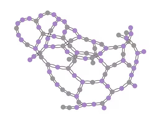
최적 컷 시각화

최적의 비트스트링으로부터 이 컷을 원래 그래프 위에 시각화할 수 있습니다.

# auxiliary function to plot graphs
def plot_result(G, x):
    colors = ["tab:grey" if i == 0 else "tab:purple" for i in x]
    pos, _default_axes = rx.spring_layout(G), plt.axes(frameon=True)
    rx.visualization.mpl_draw(
        G, node_color=colors, node_size=100, alpha=0.8, pos=pos
    )

plot_result(graph, most_likely_bitstring)

이제 컷의 값을 계산합니다:

def evaluate_sample(x: Sequence[int], graph: rx.PyGraph) -> float:
    assert len(x) == len(
        list(graph.nodes())
    ), "The length of x must coincide with the number of nodes in the graph."
    return sum(
        x[u] * (1 - x[v]) + x[v] * (1 - x[u])
        for u, v in list(graph.edge_list())
    )

cut_value = evaluate_sample(most_likely_bitstring, graph)
print("The value of the cut is:", cut_value)

The value of the cut is: 5

이렇게 작은 그래프의 경우 진정한 최적값을 무차별 대입으로 쉽게 구할 수 있으므로, QAOA 결과를 정확한 답과 비교하여 결과를 다시 확인할 수 있습니다.

# Classical baseline: enumerate all 2**n_small bitstrings and take the best cut.
def brute_force_max_cut(graph: rx.PyGraph) -> tuple[int, list[int]]:
    n = len(list(graph.nodes()))
    best_cut = -1
    best_x: list[int] = []
    for i in range(2**n):
        x = [(i >> k) & 1 for k in range(n)]
        cut = evaluate_sample(x, graph)
        if cut > best_cut:
            best_cut = int(cut)
            best_x = x
    return best_cut, best_x

classical_best, classical_x = brute_force_max_cut(graph)
print(f"Classical optimum (brute force): {classical_best}")
print(f"QAOA cut value:                  {cut_value}")

Classical optimum (brute force): 5
QAOA cut value:                  5

대규모 하드웨어 예제

IBM Quantum Platform에서 100개 이상의 Qubit을 가진 많은 장치에 접근할 수 있습니다. 100-노드 가중 그래프에서 max-cut을 해결할 장치를 하나 선택하세요. 이것은 "유틸리티 규모" 문제입니다. 워크플로는 위와 동일한 단계를 따르며, 훨씬 더 큰 그래프에 적용됩니다.

유틸리티 규모의 종단 간 워크플로

네 단계 모두 아래에 100-노드 그래프에 적용되어 표시됩니다. 구조는 소규모 설명과 동일합니다: 매핑, 트랜스파일, 실행, 사후 처리 — 다만 더 큰 문제이며 명확성을 위해 아래 네 개의 셀로 나뉘어 있습니다.

# Precomputed parity lookup table: _PARITY[b] = +1 if popcount(b) is even, else -1.
# We use this to vectorize expectation-value evaluation across all Pauli terms.
_PARITY = np.array(
    [-1 if bin(i).count("1") % 2 else 1 for i in range(256)],
    dtype=np.complex128,
)

def evaluate_sparse_pauli(state: int, observable: SparsePauliOp) -> complex:
    """Expectation value of a SparsePauliOp on a single computational-basis state.

    For a Z-only observable (which QAOA cost Hamiltonians are, after the
    QUBO-to-Hamiltonian mapping), the eigenvalue of each Pauli term on a
    computational-basis state is simply (-1)**popcount(z_mask AND state),
    i.e., the parity of the bitwise-AND of the term's Z-support and the
    measured bitstring.

    This routine packs the Z-support of every Pauli term into bytes, ANDs
    them against the measured state in a single vectorized op, and looks up
    the parity in _PARITY. For a 100-qubit / ~hundreds-of-terms Hamiltonian
    over 10_000 samples, this is dramatically faster than calling
    SparsePauliOp.expectation_value per sample.
    """
    packed_uint8 = np.packbits(observable.paulis.z, axis=1, bitorder="little")
    state_bytes = np.frombuffer(
        state.to_bytes(packed_uint8.shape[1], "little"), dtype=np.uint8
    )
    reduced = np.bitwise_xor.reduce(packed_uint8 & state_bytes, axis=1)
    return np.sum(observable.coeffs * _PARITY[reduced])

def best_solution(samples, hamiltonian):
    """Return the sampled bitstring (as int) with the lowest Hamiltonian cost."""
    min_cost = float("inf")
    min_sol = None
    for bit_str in samples.keys():
        candidate_sol = int(bit_str)
        fval = evaluate_sparse_pauli(candidate_sol, hamiltonian).real
        if fval <= min_cost:
            min_cost = fval
            min_sol = candidate_sol
    return min_sol

def _plot_cdf(objective_values: dict, ax, color):
    x_vals = sorted(objective_values.keys(), reverse=True)
    y_vals = np.cumsum([objective_values[x] for x in x_vals])
    ax.plot(x_vals, y_vals, color=color)

def plot_cdf(dist, ax, title):
    _plot_cdf(dist, ax, "C1")
    ax.vlines(min(list(dist.keys())), 0, 1, "C1", linestyle="--")
    ax.set_title(title)
    ax.set_xlabel("Objective function value")
    ax.set_ylabel("Cumulative distribution function")
    ax.grid(alpha=0.3)

def samples_to_objective_values(samples, hamiltonian):
    """Convert the samples to values of the objective function."""
    objective_values = defaultdict(float)
    for bit_str, prob in samples.items():
        candidate_sol = int(bit_str)
        fval = evaluate_sparse_pauli(candidate_sol, hamiltonian).real
        objective_values[fval] += prob
    return objective_values

Step 1: 그래프, 비용 Hamiltonian, ansatz를 구축합니다.

# Step 1: build the 100-node graph, cost Hamiltonian, and QAOA ansatz.
n_large = 100
graph_100 = rx.PyGraph()
graph_100.add_nodes_from(np.arange(0, n_large, 1))
elist = []
for edge in backend.coupling_map:
    if edge[0] < n_large and edge[1] < n_large:
        elist.append((edge[0], edge[1], 1.0))
graph_100.add_edges_from(elist)

max_cut_paulis_100 = build_max_cut_paulis(graph_100)
cost_hamiltonian_100 = SparsePauliOp.from_sparse_list(
    max_cut_paulis_100, n_large
)

circuit_100 = QAOAAnsatz(cost_operator=cost_hamiltonian_100, reps=1)
circuit_100.measure_all()

Step 2: 선택한 하드웨어 Backend에 맞게 트랜스파일합니다.

# Step 2: transpile for hardware.
pm = generate_preset_pass_manager(optimization_level=3, backend=backend)
candidate_circuit_100 = pm.run(circuit_100)

Step 3: Session 내에서 QAOA 최적화 루프를 실행한 다음 샘플링합니다.

# Step 3: run the QAOA optimization loop on the device, then sample the
# final distribution with the optimized parameters.
initial_gamma = np.pi
initial_beta = np.pi / 2
init_params = [initial_beta, initial_gamma]

objective_func_vals = []  # Global variable
with Session(backend=backend) as session:
    estimator = Estimator(mode=session)
    estimator.options.default_shots = 1000

    # Set simple error suppression/mitigation options
    estimator.options.dynamical_decoupling.enable = True
    estimator.options.dynamical_decoupling.sequence_type = "XY4"
    estimator.options.twirling.enable_gates = True
    estimator.options.twirling.num_randomizations = "auto"
    estimator.options.environment.job_tags = ["TUT_QAOA"]

    result = minimize(
        cost_func_estimator,
        init_params,
        args=(candidate_circuit_100, cost_hamiltonian_100, estimator),
        method="COBYLA",
    )
    print(result)

# Assign optimal parameters and sample the final distribution.
optimized_circuit_100 = candidate_circuit_100.assign_parameters(result.x)

sampler = Sampler(mode=backend)
sampler.options.default_shots = 10000

# Set simple error suppression/mitigation options
sampler.options.dynamical_decoupling.enable = True
sampler.options.dynamical_decoupling.sequence_type = "XY4"
sampler.options.twirling.enable_gates = True
sampler.options.twirling.num_randomizations = "auto"

# Add a unique tag to the job execution
sampler.options.environment.job_tags = ["TUT_QAOA"]

pub = (optimized_circuit_100,)
job = sampler.run([pub], shots=int(1e4))

counts_int = job.result()[0].data.meas.get_int_counts()
shots = sum(counts_int.values())
final_distribution_100_int = {
    key: val / shots for key, val in counts_int.items()
}

message: Return from COBYLA because the trust region radius reaches its lower bound.
 success: True
  status: 0
     fun: -17.172689238986344
       x: [ 2.574e+00  4.166e+00]
    nfev: 28
   maxcv: 0.0

Step 4: 샘플링된 분포를 사후 처리하여 최적 컷을 추출합니다.

# Step 4: find the best-cost sample and evaluate its cut value.
best_sol_100 = best_solution(final_distribution_100_int, cost_hamiltonian_100)
best_sol_bitstring_100 = to_bitstring(int(best_sol_100), len(graph_100))
best_sol_bitstring_100.reverse()

print("Result bitstring:", best_sol_bitstring_100)

cut_value_100 = evaluate_sample(best_sol_bitstring_100, graph_100)
print("The value of the cut is:", cut_value_100)

Result bitstring: [1, 1, 0, 1, 1, 0, 1, 1, 1, 0, 1, 0, 1, 1, 1, 0, 1, 1, 1, 1, 0, 0, 1, 0, 0, 1, 1, 0, 1, 0, 1, 0, 1, 1, 0, 1, 1, 0, 0, 0, 0, 0, 1, 1, 0, 1, 0, 0, 0, 1, 0, 0, 1, 0, 1, 0, 0, 1, 1, 1, 1, 1, 0, 1, 0, 1, 0, 0, 0, 1, 0, 1, 0, 1, 0, 0, 0, 0, 1, 0, 0, 1, 0, 1, 1, 1, 1, 0, 1, 0, 1, 0, 1, 1, 1, 0, 1, 1, 1, 0]
The value of the cut is: 156

최적화 루프에서 최소화된 비용이 수렴했는지 확인하고 결과를 시각화합니다.

# Plot convergence
plt.figure(figsize=(12, 6))
plt.plot(objective_func_vals)
plt.xlabel("Iteration")
plt.ylabel("Cost")
plt.show()

# Visualize the cut
plot_result(graph_100, best_sol_bitstring_100)

# Plot cumulative distribution function
result_dist = samples_to_objective_values(
    final_distribution_100_int, cost_hamiltonian_100
)
fig, ax = plt.subplots(1, 1, figsize=(8, 6))
plot_cdf(result_dist, ax, backend.name)

다음 단계

이 작업이 흥미로웠다면 다음 자료에 관심이 있을 수 있습니다:

추천

• QAOA를 위한 고급 기법 — QAOA 성능을 향상시키기 위한 고급 전략을 살펴봅니다
• 다목적 최적화 챌린지 — 다목적 양자 최적화에 관한 이 커뮤니티 챌린지로 실력을 시험해 보세요
• 미세한 Circuit 최적화 조정을 위한 트랜스파일 문서
• 하드웨어 결과 개선을 위한 오류 억제 및 완화