페르미온 격자 모델의 샘플 기반 Krylov 양자 대각화
사용 시간 추정: Heron r2 프로세서에서 약 9초 (참고: 이는 추정값이며 실제 실행 시간은 다를 수 있습니다.)
학습 성과
이 튜토리얼을 마치면 다음을 이해할 수 있습니다:
- 양자 처리 장치(QPU)에서 샘플링한 비트열을 사용하여 격자 모델의 바닥 상태 에너지를 근사하기 위해 SQD Qiskit 애드온을 사용하는 방법.
- 페르미온 시뮬레이션을 위한 시간 진화 Circuit을 구성하기 위해 ffsim을 사용하는 방법.
- 샘플 기반 Krylov 대각화(SQKD) 알고리즘으로 후처리하기 위해 여러 Circuit의 샘플을 결합하는 방법.
사전 요구 사항
이 튜토리얼을 진행하기 전에 다음 주제에 익숙할 것을 권장합니다:
배경
이 튜토리얼은 샘플 기반 양자 대각화(SQD)를 사용하여 페르미온 격자 모델의 바닥 상태 에너지를 추정하는 방법을 설명합니다. 구체적으로, 금속 내에 삽입된 자기 불순물을 기술하는 데 사용되는 1차원 단일 불순물 앤더슨 모델(SIAM)을 연구합니다.
이 튜토리얼은 관련 튜토리얼 화학 해밀토니안의 샘플 기반 양자 대각화와 유사한 워크플로를 따릅니다. 그러나 양자 회로를 구성하는 방법에서 중요한 차이가 있습니다. 다른 튜토리얼은 잠재적으로 수백만 개의 상호작용 항을 가진 화학 해밀토니안에 적합한 휴리스틱 변분 앤자츠를 사용합니다. 반면, 이 튜토리얼은 해밀토니안에 의한 시간 진화를 근사하는 회로를 사용합니다. 이러한 회로는 깊이가 깊을 수 있어, 격자 모델 응용에 더 적합합니다. 이 회로들이 준비하는 상태 벡터들은 Krylov 부분공간의 기저를 형성하며, 그 결과 적절한 가정 하에서 알고리즘은 바닥 상태로 증명 가능하고 효율적으로 수렴합니다.
이 튜토리얼에서 사용하는 방법은 SQD와 Krylov 양자 대각화(KQD)에서 사용하는 기법의 결합으로 볼 수 있습니다. 이 결합 방법은 때때로 샘플 기반 Krylov 양자 대각화(SQKD)라고 불립니다. KQD 방법에 대한 튜토리얼은 격자 해밀토니안의 Krylov 양자 대각화를 참조하세요.
이 튜토리얼은 논문 "Quantum-Centric Algorithm for Sample-Based Krylov Diagonalization"을 기반으로 하며, 더 자세한 내용은 해당 논문을 참조할 수 있습니다.
단일 불순물 앤더슨 모델(SIAM)
1차원 SIAM 해밀토니안은 세 항의 합입니다:
여기서
여기서 는 스핀 를 가진 배스 사이트에 대한 페르미온 생성/소멸 연산자이고, 는 불순물 모드에 대한 생성/소멸 연산자이며, 입니다. , , 는 각각 호핑, 온-사이트, 혼성화 상호작용을 나타내는 실수이고, 는 화학 퍼텐셜을 지정하는 실수입니다.
해밀토니안이 일반적인 상호작용-전자 해밀토니안의 특정 사례임에 유의하세요:
여기서 은 페르미온 생성 및 소멸 연산자에 대해 이차식인 일체 항들로 구성되고, 는 사차식인 이체 항들로 구성됩니다. SIAM의 경우,
이고 은 해밀토니안의 나머지 항들을 포함합니다. 해밀토니안을 프로그래밍 방식으로 표현하기 위해 행렬 와 텐서 를 저장합니다.
위치 기저와 운동량 기저
의 근사적 병진 대칭성으로 인해, 위치 기저(위에서 해밀토니안이 지정된 오비탈 기저)에서는 바닥 상태가 희소하지 않을 것으로 예상됩니다. SQD의 성능은 바닥 상태가 희소한 경우, 즉 소수의 계산 기저 상태에만 유의미한 가중치를 가지는 경우에만 보장됩니다. 바닥 상태의 희소성을 개선하기 위해 가 대각화되는 오비탈 기저에서 시뮬레이션을 수행합니다. 이 기저를 운동량 기저라고 합니다. 는 이차 페르미온 해밀토니안이므로 오비탈 회전에 의해 효율적으로 대각화될 수 있습니다.
해밀토니안에 의한 근사 시간 진화
해밀토니안에 의한 시간 진화를 근사하기 위해 2차 Trotter-Suzuki 분해를 사용합니다:
Jordan-Wigner 변환 하에서, 에 의한 시간 진화는 불순물 사이트의 스핀업 및 스핀다운 오비탈 사이의 단일 CPhase Gate에 해당합니다. 은 이차 페르미온 해밀토니안이므로 에 의한 시간 진화는 오비탈 회전에 해당합니다.
Krylov 기저 상태 (여기서 는 Krylov 부분공간의 차원)은 단일 Trotter 스텝의 반복 적용으로 형성되므로
다음의 SQD 기반 워크플로에서는 이 회로 집합에서 샘플링하고 SQD로 결합된 비트열 집합을 후처리합니다. 이 방법은 관련 튜토리얼 화학 해밀토니안의 샘플 기반 양자 대각화에서 사용된 방법, 즉 단일 휴리스틱 변분 Circuit에서 샘플을 추출하는 방식과 대조됩니다.
요구 사항
이 튜토리얼을 시작하기 전에 다음이 설치되어 있는지 확인하세요:
- Qiskit SDK v1.0 이상 (시각화 지원 포함)
- Qiskit Runtime v0.22 이상 (
pip install qiskit-ibm-runtime) - SQD Qiskit 애드온 v0.11 이상 (
pip install qiskit-addon-sqd) - ffsim v0.0.72 이상 (
pip install ffsim)
소규모 시뮬레이터 예제
1단계: 문제를 양자 Circuit으로 매핑하기
먼저 위치 기저에서 SIAM 해밀토니안을 생성합니다. 해밀토니안은 행렬 와 텐서 로 표현됩니다. 그런 다음 운동량 기저로 회전합니다. 위치 기저에서는 불순물을 첫 번째 사이트에 배치합니다. 그러나 운동량 기저로 회전할 때는 다른 오비탈과의 상호작용을 용이하게 하기 위해 불순물을 중앙 사이트로 이동합니다.
# Added by doQumentation — required packages for this notebook
!pip install -q ffsim matplotlib numpy pyscf qiskit qiskit-addon-sqd qiskit-ibm-runtime scipy
import numpy as np
import pyscf.fci

def siam_hamiltonian(
    norb: int,
    hopping: float,
    onsite: float,
    hybridization: float,
    chemical_potential: float,
) -> tuple[np.ndarray, np.ndarray]:
    """Hamiltonian for the single-impurity Anderson model."""
    # Place the impurity on the first site
    impurity_orb = 0

    # One body matrix elements in the "position" basis
    h1e = np.zeros((norb, norb))
    np.fill_diagonal(h1e[:, 1:], -hopping)
    np.fill_diagonal(h1e[1:, :], -hopping)
    h1e[impurity_orb, impurity_orb + 1] = -hybridization
    h1e[impurity_orb + 1, impurity_orb] = -hybridization
    h1e[impurity_orb, impurity_orb] = chemical_potential

    # Two body matrix elements in the "position" basis
    h2e = np.zeros((norb, norb, norb, norb))
    h2e[impurity_orb, impurity_orb, impurity_orb, impurity_orb] = onsite

    return h1e, h2e

def momentum_basis(norb: int) -> np.ndarray:
    """Get the orbital rotation to change from the position to the momentum basis."""
    n_bath = norb - 1

    # Orbital rotation that diagonalizes the bath (non-interacting system)
    hopping_matrix = np.zeros((n_bath, n_bath))
    np.fill_diagonal(hopping_matrix[:, 1:], -1)
    np.fill_diagonal(hopping_matrix[1:, :], -1)
    _, vecs = np.linalg.eigh(hopping_matrix)

    # Expand to include impurity
    orbital_rotation = np.zeros((norb, norb))
    # Impurity is on the first site
    orbital_rotation[0, 0] = 1
    orbital_rotation[1:, 1:] = vecs

    # Move the impurity to the center
    new_index = n_bath // 2
    perm = np.r_[1 : (new_index + 1), 0, (new_index + 1) : norb]
    orbital_rotation = orbital_rotation[:, perm]

    return orbital_rotation

def rotated(
    h1e: np.ndarray, h2e: np.ndarray, orbital_rotation: np.ndarray
) -> tuple[np.ndarray, np.ndarray]:
    """Rotate the orbital basis of a Hamiltonian."""
    h1e_rotated = np.einsum(
        "ab,Aa,Bb->AB",
        h1e,
        orbital_rotation,
        orbital_rotation.conj(),
        optimize="greedy",
    )
    h2e_rotated = np.einsum(
        "abcd,Aa,Bb,Cc,Dd->ABCD",
        h2e,
        orbital_rotation,
        orbital_rotation.conj(),
        orbital_rotation,
        orbital_rotation.conj(),
        optimize="greedy",
    )
    return h1e_rotated, h2e_rotated

# Total number of spatial orbitals, including the bath sites and the impurity
# This should be an even number
norb = 8

# System is half-filled
nelec = (norb // 2, norb // 2)
# One orbital is the impurity, the rest are bath sites
n_bath = norb - 1

# Hamiltonian parameters
hybridization = 1.0
hopping = 1.0
onsite = 10.0
chemical_potential = -0.5 * onsite

# Generate Hamiltonian in position basis
h1e, h2e = siam_hamiltonian(
    norb=norb,
    hopping=hopping,
    onsite=onsite,
    hybridization=hybridization,
    chemical_potential=chemical_potential,
)

# Rotate to momentum basis
orbital_rotation = momentum_basis(norb)
h1e_momentum, h2e_momentum = rotated(h1e, h2e, orbital_rotation.T.conj())
# In the momentum basis, the impurity is placed in the center
impurity_index = n_bath // 2

# Use PySCF to compute the exact ground state energy
reference_energy, _ = pyscf.fci.direct_spin1.kernel(h1e, h2e, norb, nelec)
from typing import Sequence

import ffsim
import scipy
from qiskit import QuantumCircuit, QuantumRegister
from qiskit.circuit import CircuitInstruction, Qubit
from qiskit.circuit.library import CPhaseGate, XGate, XXPlusYYGate

def prepare_initial_state(qubits: Sequence[Qubit], norb: int, nocc: int):
    """Prepare initial state."""
    assert norb >= 8
    x_gate = XGate()
    rot = XXPlusYYGate(0.5 * np.pi, -0.5 * np.pi)
    for i in range(nocc):
        yield CircuitInstruction(x_gate, [qubits[i]])
        yield CircuitInstruction(x_gate, [qubits[norb + i]])
    for i in range(3):
        for j in range(nocc - i - 1, nocc + i, 2):
            yield CircuitInstruction(rot, [qubits[j], qubits[j + 1]])
            yield CircuitInstruction(
                rot, [qubits[norb + j], qubits[norb + j + 1]]
            )
    yield CircuitInstruction(rot, [qubits[j + 1], qubits[j + 2]])
    yield CircuitInstruction(
        rot, [qubits[norb + j + 1], qubits[norb + j + 2]]
    )

def trotter_step(
    qubits: Sequence[Qubit],
    time_step: float,
    one_body_evolution: np.ndarray,
    h2e: np.ndarray,
    impurity_index: int,
    norb: int,
):
    """A Trotter step."""
    # Assume the two-body interaction is just the on-site interaction of the impurity
    onsite = h2e[
        impurity_index, impurity_index, impurity_index, impurity_index
    ]
    # Two-body evolution for half the time
    yield CircuitInstruction(
        CPhaseGate(-0.5 * time_step * onsite),
        [qubits[impurity_index], qubits[norb + impurity_index]],
    )
    # One-body evolution for the full time
    yield CircuitInstruction(
        ffsim.qiskit.OrbitalRotationJW(norb, one_body_evolution), qubits
    )
    # Two-body evolution for half the time
    yield CircuitInstruction(
        CPhaseGate(-0.5 * time_step * onsite),
        [qubits[impurity_index], qubits[norb + impurity_index]],
    )

# Time step
time_step = 0.2
# Number of Krylov basis states
krylov_dim = 8

# Initialize circuit
qubits = QuantumRegister(2 * norb, name="q")
circuit = QuantumCircuit(qubits)

# Generate initial state
for instruction in prepare_initial_state(qubits, norb=norb, nocc=norb // 2):
    circuit.append(instruction)
circuit.measure_all()

# Create list of circuits, starting with the initial state circuit
circuits = [circuit.copy()]

# Add time evolution circuits to the list
one_body_evolution = scipy.linalg.expm(-1j * time_step * h1e_momentum)
for i in range(krylov_dim - 1):
    # Remove measurements
    circuit.remove_final_measurements()
    # Append another Trotter step
    for instruction in trotter_step(
        qubits,
        time_step,
        one_body_evolution,
        h2e_momentum,
        impurity_index,
        norb,
    ):
        circuit.append(instruction)
    # Measure qubits
    circuit.measure_all()
    # Add a copy of the circuit to the list
    circuits.append(circuit.copy())
다음으로, Krylov 기저 상태를 생성하는 Circuit들을 만듭니다. 각 스핀 종에 대해, 초기 상태 는 상태 에서 시작하여 페르미 준위에 가장 가까운 세 전자를 가장 가까운 4개의 빈 모드로 가능한 모든 여기시키는 중첩으로 주어지며, 일곱 개의 XXPlusYYGate의 적용으로 구현됩니다. 시간 진화된 상태들은 2차 Trotter 스텝의 연속 적용으로 생성됩니다.
이 모델과 Circuit 설계 방법에 대한 더 자세한 설명은 "Quantum-Centric Algorithm for Sample-Based Krylov Diagonalization"을 참조하세요.
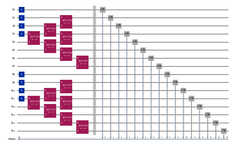
circuits[0].draw("mpl", scale=0.4, fold=-1)
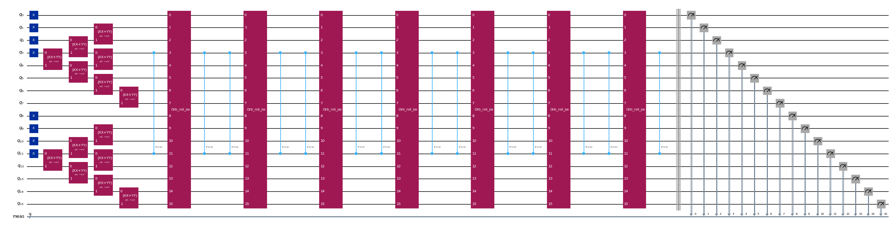
circuits[-1].draw("mpl", scale=0.4, fold=-1)
Step 2: 양자 실행을 위한 문제 최적화
다음으로, 대상 하드웨어에 맞게 Circuit을 최적화합니다. 지금은 지정된 큐비트 수와 시간 진화 Circuit이 자연스럽게 분해되는 게이트 세트를 가진 일반 Backend를 생성합니다.
from qiskit.providers.fake_provider import GenericBackendV2

backend = GenericBackendV2(
    2 * norb, basis_gates=["cp", "xx_plus_yy", "p", "x"]
)
이제 Qiskit을 사용하여 Circuit을 대상 Backend로 트랜스파일합니다.
from qiskit.transpiler import generate_preset_pass_manager

pass_manager = generate_preset_pass_manager(
    optimization_level=3, backend=backend
)
isa_circuits = pass_manager.run(circuits)
Step 3: Qiskit 프리미티브를 사용한 실행
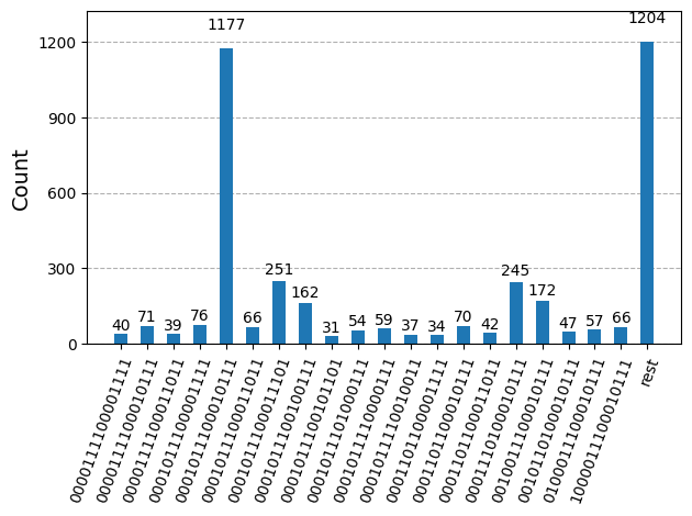
하드웨어 실행을 위해 Circuit을 최적화한 후, 대상 하드웨어에서 실행하여 바닥 상태 에너지 추정을 위한 샘플을 수집할 준비가 되었습니다. Sampler 프리미티브를 사용하여 각 Circuit에서 비트 문자열을 샘플링한 뒤, 모든 결과를 단일 counts 딕셔너리로 합산하고 가장 많이 샘플링된 상위 20개 비트 문자열을 도식화합니다.
from qiskit.visualization import plot_histogram
from qiskit.primitives import StatevectorSampler

# Sample from the circuits
sampler = StatevectorSampler()
job = sampler.run(isa_circuits, shots=500)
from qiskit.primitives import BitArray

# Combine the shots from the individual Trotter circuits
bit_array = BitArray.concatenate_shots(
    [result.data.meas for result in job.result()]
)

plot_histogram(bit_array.get_counts(), number_to_keep=20)
Step 4: 후처리 및 원하는 고전 형식으로 결과 반환
이제 diagonalize_fermionic_hamiltonian 함수를 사용하여 SQD 알고리즘을 실행합니다. 이 함수의 인수에 대한 설명은 API 문서를 참고하세요.
from qiskit_addon_sqd.fermion import (
    SCIResult,
    diagonalize_fermionic_hamiltonian,
)

# List to capture intermediate results
result_history = []

def callback(results: list[SCIResult]):
    result_history.append(results)
    iteration = len(result_history)
    print(f"Iteration {iteration}")
    for i, result in enumerate(results):
        print(f"\tSubsample {i}")
        print(f"\t\tEnergy: {result.energy}")
        print(
            f"\t\tSubspace dimension: {np.prod(result.sci_state.amplitudes.shape)}"
        )

rng = np.random.default_rng(24)
result = diagonalize_fermionic_hamiltonian(
    h1e_momentum,
    h2e_momentum,
    bit_array,
    samples_per_batch=100,
    norb=norb,
    nelec=nelec,
    num_batches=3,
    max_iterations=5,
    symmetrize_spin=True,
    callback=callback,
    seed=rng,
)
Iteration 1
	Subsample 0
		Energy: -13.4222953188441
		Subspace dimension: 529
	Subsample 1
		Energy: -13.42237556285828
		Subspace dimension: 784
	Subsample 2
		Energy: -13.422045397387413
		Subspace dimension: 529
Iteration 2
	Subsample 0
		Energy: -13.422379583305478
		Subspace dimension: 900
	Subsample 1
		Energy: -13.422376197704326
		Subspace dimension: 841
	Subsample 2
		Energy: -13.422421162849295
		Subspace dimension: 1089
Iteration 3
	Subsample 0
		Energy: -13.422421164670345
		Subspace dimension: 1156
	Subsample 1
		Energy: -13.422421492737689
		Subspace dimension: 1156
	Subsample 2
		Energy: -13.422421205869572
		Subspace dimension: 1156
Iteration 4
	Subsample 0
		Energy: -13.422421494558726
		Subspace dimension: 1225
	Subsample 1
		Energy: -13.422421492737689
		Subspace dimension: 1156
	Subsample 2
		Energy: -13.422421492737689
		Subspace dimension: 1156
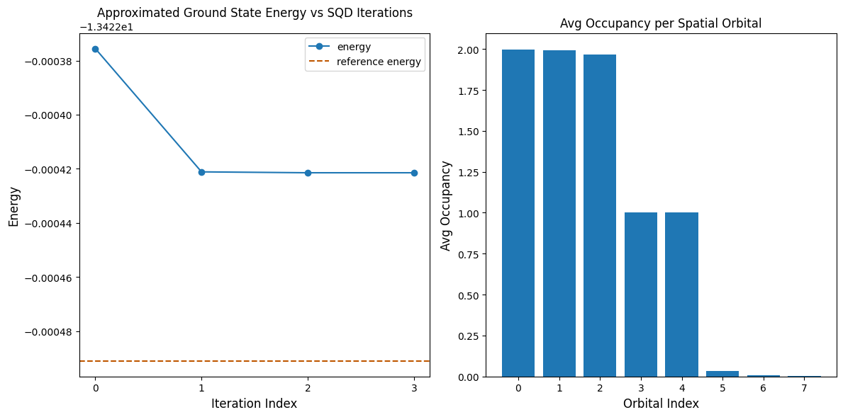
다음 코드 셀은 결과를 도식화합니다. 첫 번째 그래프는 형상 복원 반복 횟수에 따른 계산된 에너지를 나타내고, 두 번째 그래프는 마지막 반복 후 각 공간 오비탈의 평균 점유율을 보여줍니다. 이 문제는 매우 소규모이므로, 첫 번째 반복에서 이미 정확한 에너지에 매우 근접합니다(y축의 스케일에 주목하세요).
import matplotlib.pyplot as plt

min_es = [
    min(result, key=lambda res: res.energy).energy
    for result in result_history
]
min_id, min_e = min(enumerate(min_es), key=lambda x: x[1])

# Data for energies plot
x1 = range(len(result_history))

# Data for avg spatial orbital occupancy
y2 = np.sum(result.orbital_occupancies, axis=0)
x2 = range(len(y2))

fig, axs = plt.subplots(1, 2, figsize=(12, 6))

# Plot energies
axs[0].plot(x1, min_es, label="energy", marker="o")
axs[0].set_xticks(x1)
axs[0].set_xticklabels(x1)
axs[0].axhline(
    y=reference_energy,
    color="#BF5700",
    linestyle="--",
    label="reference energy",
)
axs[0].set_title("Approximated Ground State Energy vs SQD Iterations")
axs[0].set_xlabel("Iteration Index", fontdict={"fontsize": 12})
axs[0].set_ylabel("Energy", fontdict={"fontsize": 12})
axs[0].legend()

# Plot orbital occupancy
axs[1].bar(x2, y2, width=0.8)
axs[1].set_xticks(x2)
axs[1].set_xticklabels(x2)
axs[1].set_title("Avg Occupancy per Spatial Orbital")
axs[1].set_xlabel("Orbital Index", fontdict={"fontsize": 12})
axs[1].set_ylabel("Avg Occupancy", fontdict={"fontsize": 12})

print(f"Reference energy: {reference_energy:.5f}")
print(f"SQD energy: {min_e:.5f}")
print(f"Absolute error: {abs(min_e - reference_energy):.5f}")
plt.tight_layout()
plt.show()
Reference energy: -13.42249
SQD energy: -13.42242
Absolute error: 0.00007
에너지 검증
SQD가 반환하는 에너지는 실제 바닥 상태 에너지의 상한값임이 보장됩니다. SQD는 바닥 상태를 근사하는 상태 벡터의 계수도 함께 반환하기 때문에 에너지 값을 검증할 수 있습니다. 다음 코드 셀에서 시연하듯이, 일체 및 이체 환산 밀도 행렬을 사용하여 상태 벡터로부터 에너지를 계산할 수 있습니다.
rdm1 = result.sci_state.rdm(rank=1, spin_summed=True)
rdm2 = result.sci_state.rdm(rank=2, spin_summed=True)

energy = np.sum(h1e_momentum * rdm1) + 0.5 * np.sum(h2e_momentum * rdm2)

print(f"Recomputed energy: {energy:.5f}")
Recomputed energy: -13.42242
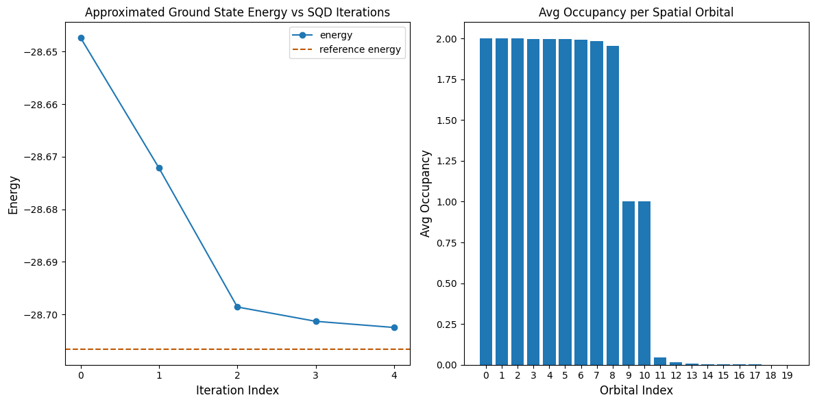
대규모 하드웨어 예제
이제 실제 QPU에서 더 큰 예제를 실행합니다. 참조 에너지로는 별도로 수행한 DMRG 계산 결과를 사용합니다.
from qiskit_ibm_runtime import SamplerV2 as Sampler
from qiskit_ibm_runtime import QiskitRuntimeService

# Model parameters
norb = 20
nelec = (norb // 2, norb // 2)
n_bath = norb - 1
hybridization = 1.0
hopping = 1.0
onsite = 10.0
chemical_potential = -0.5 * onsite

# Generate Hamiltonian and orbital rotation
h1e, h2e = siam_hamiltonian(
    norb=norb,
    hopping=hopping,
    onsite=onsite,
    hybridization=hybridization,
    chemical_potential=chemical_potential,
)
orbital_rotation = momentum_basis(norb)
h1e_momentum, h2e_momentum = rotated(h1e, h2e, orbital_rotation.T.conj())
impurity_index = n_bath // 2

# Set reference energy to DMRG value computed separately
reference_energy = -28.70659686

# Algorithm parameters
time_step = 0.2
krylov_dim = 8

# Construct circuits
qubits = QuantumRegister(2 * norb, name="q")
circuit = QuantumCircuit(qubits)
for instruction in prepare_initial_state(qubits, norb=norb, nocc=norb // 2):
    circuit.append(instruction)
circuit.measure_all()
circuits = [circuit.copy()]
one_body_evolution = scipy.linalg.expm(-1j * time_step * h1e_momentum)
for i in range(krylov_dim - 1):
    circuit.remove_final_measurements()
    for instruction in trotter_step(
        qubits,
        time_step,
        one_body_evolution,
        h2e_momentum,
        impurity_index,
        norb,
    ):
        circuit.append(instruction)
    circuit.measure_all()
    circuits.append(circuit.copy())

# Initialize hardware backend
service = QiskitRuntimeService()
backend = service.least_busy(
    operational=True, simulator=False, min_num_qubits=127
)
print(f"Using backend {backend.name}")

# Transpile to backend
pass_manager = generate_preset_pass_manager(
    optimization_level=3, backend=backend
)
isa_circuits = pass_manager.run(circuits)

# Sample from the circuits
sampler = Sampler(backend)
sampler.options.environment.job_tags = ["TUT_SKQD"]
job = sampler.run(isa_circuits, shots=500)

# Combine the shots from the individual Trotter circuits
bit_array = BitArray.concatenate_shots(
    [result.data.meas for result in job.result()]
)

# Run configuration recovery and diagonalization
result_history = []

def callback(results: list[SCIResult]):
    result_history.append(results)
    iteration = len(result_history)
    print(f"Iteration {iteration}")
    for i, result in enumerate(results):
        print(f"\tSubsample {i}")
        print(f"\t\tEnergy: {result.energy}")
        print(
            f"\t\tSubspace dimension: {np.prod(result.sci_state.amplitudes.shape)}"
        )

rng = np.random.default_rng(24)
result = diagonalize_fermionic_hamiltonian(
    h1e_momentum,
    h2e_momentum,
    bit_array,
    samples_per_batch=100,
    norb=norb,
    nelec=nelec,
    num_batches=3,
    max_iterations=5,
    symmetrize_spin=True,
    callback=callback,
    seed=rng,
)

# Plot results
min_es = [
    min(result, key=lambda res: res.energy).energy
    for result in result_history
]
min_id, min_e = min(enumerate(min_es), key=lambda x: x[1])
x1 = range(len(result_history))
y2 = np.sum(result.orbital_occupancies, axis=0)
x2 = range(len(y2))
fig, axs = plt.subplots(1, 2, figsize=(12, 6))
axs[0].plot(x1, min_es, label="energy", marker="o")
axs[0].set_xticks(x1)
axs[0].set_xticklabels(x1)
axs[0].axhline(
    y=reference_energy,
    color="#BF5700",
    linestyle="--",
    label="reference energy",
)
axs[0].set_title("Approximated Ground State Energy vs SQD Iterations")
axs[0].set_xlabel("Iteration Index", fontdict={"fontsize": 12})
axs[0].set_ylabel("Energy", fontdict={"fontsize": 12})
axs[0].legend()
axs[1].bar(x2, y2, width=0.8)
axs[1].set_xticks(x2)
axs[1].set_xticklabels(x2)
axs[1].set_title("Avg Occupancy per Spatial Orbital")
axs[1].set_xlabel("Orbital Index", fontdict={"fontsize": 12})
axs[1].set_ylabel("Avg Occupancy", fontdict={"fontsize": 12})
print(f"Reference energy: {reference_energy:.5f}")
print(f"SQD energy: {min_e:.5f}")
print(f"Absolute error: {abs(min_e - reference_energy):.5f}")
plt.tight_layout()
plt.show()
Using backend ibm_boston
Iteration 1
	Subsample 0
		Energy: -28.63965951544449
		Subspace dimension: 9801
	Subsample 1
		Energy: -28.625588929202006
		Subspace dimension: 9409
	Subsample 2
		Energy: -28.647371834135498
		Subspace dimension: 8281
Iteration 2
	Subsample 0
		Energy: -28.67213260849567
		Subspace dimension: 29584
	Subsample 1
		Energy: -28.670340686158816
		Subspace dimension: 27225
	Subsample 2
		Energy: -28.669976379525988
		Subspace dimension: 31329
Iteration 3
	Subsample 0
		Energy: -28.68622875601382
		Subspace dimension: 36100
	Subsample 1
		Energy: -28.698569623143126
		Subspace dimension: 34225
	Subsample 2
		Energy: -28.694848533971882
		Subspace dimension: 33856
Iteration 4
	Subsample 0
		Energy: -28.69883392844593
		Subspace dimension: 42025
	Subsample 1
		Energy: -28.701289495200996
		Subspace dimension: 38025
	Subsample 2
		Energy: -28.699319594978245
		Subspace dimension: 45369
Iteration 5
	Subsample 0
		Energy: -28.701936886834154
		Subspace dimension: 51076
	Subsample 1
		Energy: -28.702468711812013
		Subspace dimension: 53824
	Subsample 2
		Energy: -28.702298147575938
		Subspace dimension: 52900
Reference energy: -28.70660
SQD energy: -28.70247
Absolute error: 0.00413
다음 단계
이 작업이 흥미로우셨다면, 다음 자료들도 관심을 가질 수 있습니다:
- 화학 해밀토니안의 샘플 기반 양자 대각화 - Trotter Circuit 대신 휴리스틱 변분 앤자츠를 사용하는 관련 튜토리얼
- 격자 해밀토니안의 Krylov 양자 대각화 - KQD 방법에 관한 튜토리얼
- SQD 애드온 API 문서 -
diagonalize_fermionic_hamiltonian함수 참고 자료 - Quantum-Centric Algorithm for Sample-Based Krylov Diagonalization - 이 튜토리얼의 기반이 된 논문