Optimization Mapper Qiskit 애드온으로 QAOA 웜스타트하기

사용량 추정치: Heron r3에서 9분 (참고: 이는 추정치일 뿐입니다. 실제 실행 시간은 다를 수 있습니다.)

학습 목표

• qiskit-addon-opt-mapper를 사용하여 max-cut 문제를 양자 이차 무제약 이진 최적화(QUBO) 형식으로 매핑하는 방법

• 시뮬레이터에서 표준 QAOA를 구현하고 실행하는 방법

• 이차 프로그램(QP) 완화를 계산하고 웜스타트 회로를 구성하여 WS-QAOA를 적용하는 방법

• 표준 QAOA와 WS-QAOA 간의 에너지 수렴 및 해의 품질을 비교하는 방법

사전 필요 사항

• QAOA 튜토리얼

• 고급 QAOA 튜토리얼

배경

양자 근사 최적화 알고리즘(QAOA)은 max-cut 및 일반적인 QUBO 형식과 같은 조합 최적화 문제를 해결하도록 설계된 하이브리드 양자-고전 알고리즘입니다. Qiskit에서 QAOA에 대한 기초적인 소개는 QAOA 튜토리얼을, 더 고급의 회로 구성 기법은 고급 QAOA 튜토리얼을 참조하세요.

표준 QAOA에서는:

• 초기 상태는 균일 중첩 $|+\rangle^{\otimes n}$입니다.
• 변분 매개변수는 무작위로 초기화됩니다.
• 고전 최적화기가 비용 함수를 최소화하는 매개변수를 탐색합니다.

하지만 실제적인 문제 크기와 노이즈가 있는 양자 하드웨어에서는 무작위 초기화 때문에 수렴이 느려지고, 좋지 않은 국소 최솟값에 갇히며, 최적화 비용이 커질 수 있습니다.

웜스타트 QAOA(WS-QAOA)는 고전 최적화 통찰을 양자 회로에 직접 통합하여 이를 개선합니다. 이 튜토리얼은 Egger, Mareček, Woerner가 Warm-starting quantum optimization에서 소개한 방법을 따릅니다. 핵심 아이디어는 다음과 같습니다:

1. 원래 이진 문제의 연속 완화($\{0,1\}^n$ 대신 $[0,1]^n$에 대한 이차 프로그램)를 풉니다.

2. 완화된 해 $c^*_i \in [0,1]$를 $Y$-회전 각도 $\theta_i = 2\arcsin(\sqrt{c^*_i})$를 사용하여 사용자 정의 초기 상태로 인코딩하여, 큐비트 $i$가 $|1\rangle$을 측정할 확률이 $c^*_i$인 상태에서 시작하도록 합니다.

3. 바닥 상태가 웜스타트 초기 상태인 사용자 정의 믹서로 표준 $X$-믹서를 대체하여, 알고리즘이 고전적 해 근처에서 시작하고 그 주변을 탐색할 수 있도록 합니다.

정규화 매개변수 $\varepsilon \in [0, 0.5]$는 도달 가능성 문제를 피하기 위해 $c^*_i$를 0과 1로부터 떨어뜨려 클리핑합니다. $|0\rangle$ 또는 $|1\rangle$로 초기화된 큐비트는 비용 해밀토니안에 의해 이동될 수 없습니다. $\varepsilon = 0.5$에서 WS-QAOA는 정확히 표준 QAOA로 환원됩니다.

문제 모델링은 qiskit-addon-opt-mapper 패키지를 사용하며, 이 패키지의 Maxcut 애플리케이션 클래스는 그래프로부터 직접 QUBO를 구성하고, 변환기(converter)와 번역기(translator)는 결과 문제를 양자 해밀토니안으로 매핑합니다.

요구 사항

이 튜토리얼을 시작하기 전에 다음이 설치되어 있는지 확인하세요:

• 시각화 지원이 포함된 Qiskit SDK v2.0 이상

• Qiskit Runtime v0.43 이상 (pip install qiskit-ibm-runtime)

• Optimization Mapper Qiskit 애드온 (pip install qiskit-addon-opt-mapper)

• SciPy (pip install scipy)

• NetworkX (pip install networkx)

설정

이 튜토리얼 전반에서 사용되는 필요한 모든 라이브러리를 임포트하고 헬퍼 함수를 정의합니다.

# Added by doQumentation — required packages for this notebook
!pip install -q matplotlib networkx numpy qiskit qiskit-addon-opt-mapper qiskit-ibm-runtime scipy

import numpy as np
import matplotlib.pyplot as plt
import networkx as nx
from scipy.optimize import minimize

from qiskit.circuit import QuantumCircuit, ParameterVector
from qiskit.circuit.library import qaoa_ansatz
from qiskit.quantum_info import Statevector
from qiskit.primitives import StatevectorEstimator, StatevectorSampler
from qiskit.transpiler.preset_passmanagers import generate_preset_pass_manager
from qiskit_ibm_runtime import (
    QiskitRuntimeService,
    Session,
    EstimatorOptions,
    EstimatorV2 as Estimator,
    SamplerV2 as Sampler,
)

from qiskit_addon_opt_mapper.applications import Maxcut
from qiskit_addon_opt_mapper.converters import OptimizationProblemToQubo
from qiskit_addon_opt_mapper.translators import to_ising

소규모 시뮬레이터 예제

이 튜토리얼 전반에서 사용할 예제로 가중 그래프의 소규모 max-cut 문제를 다룹니다. Max-cut은 다음과 같이 묻습니다: 엣지 가중치가 $w_{ij}$인 그래프 $G=(V,E)$가 주어졌을 때, 컷을 가로지르는 엣지의 총 가중치를 최대화하는 정점들의 두 집합 $S$와 $\bar{S}$로의 분할을 찾으세요.

QUBO 최소화 문제로서 max-cut은 다음과 같이 쓸 수 있습니다: $\min_{x \in \{0,1\}^n} -\sum_{(i,j) \in E} w_{ij}(x_i + x_j - 2x_i x_j)$

시뮬레이터에서 다루기 쉽도록 4개 노드로 이루어진 그래프를 사용합니다.

단계 1: 고전 입력을 양자 문제로 매핑하기

qiskit-addon-opt-mapper의 Maxcut 애플리케이션 클래스를 사용하여 max-cut 문제를 정의하며, 이 클래스는 그래프로부터 직접 QUBO 형식을 구성합니다. 그런 다음 이를 QUBO로 변환하고 QAOA에 적합한 이징 해밀토니안(SparsePauliOp)으로 번역합니다. 또한 웜스타트 초기점 $c^*$를 얻기 위해 QUBO의 연속 완화 — 이진 제약 $x_i \in \{0,1\}$을 $x_i \in [0,1]$로 대체 — 를 풉니다.

# Define a 4-node weighted graph for the max-cut problem
n_nodes = 4
edges = [(0, 1, 1.0), (0, 2, 1.0), (1, 2, 1.0), (1, 3, 1.0), (2, 3, 1.0)]

G = nx.Graph()
G.add_nodes_from(range(n_nodes))
G.add_weighted_edges_from(edges)

pos = nx.spring_layout(G, seed=42)
edge_labels = {(u, v): d["weight"] for u, v, d in G.edges(data=True)}

fig, ax = plt.subplots(figsize=(4, 3))
nx.draw(G, pos, with_labels=True, node_color="lightblue", ax=ax)
nx.draw_networkx_edge_labels(G, pos, edge_labels=edge_labels, ax=ax)
ax.set_title("Max-Cut graph")
plt.tight_layout()
plt.show()

이 그래프에는 다섯 개의 엣지가 있습니다. 최적의 max-cut은 노드를 $S = \{0, 3\}$과 $\bar{S} = \{1, 2\}$로 분할하여(또는 그 여집합) 다섯 개의 엣지 중 네 개를 절단하며, 컷 값은 4입니다.

# Build the max-cut problem directly from the NetworkX graph using the
# Maxcut application class. Internally it constructs the QUBO
#   minimize  -sum_{(i,j) in E} w_ij * (x_i + x_j - 2*x_i*x_j)
# (each edge contributes -w to the linear terms and +2w to the quadratic
# term), so we get the same OptimizationProblem without the boilerplate.
maxcut = Maxcut(G)
prob = maxcut.to_optimization_problem()
print(prob.prettyprint())

Problem name: Max-cut

Maximize
  -2*x_0*x_1 - 2*x_0*x_2 - 2*x_1*x_2 - 2*x_1*x_3 - 2*x_2*x_3 + 2*x_0 + 3*x_1
  + 3*x_2 + 2*x_3

Subject to
  No constraints

  Binary variables (4)
    x_0 x_1 x_2 x_3

Maxcut 클래스는 QUBO 구성을 감싸주므로 max-cut 목적 함수를 직접 전개할 필요가 없습니다. 출력된 목적 함수는 각 변수의 선형 계수(개별적으로 컷에 얼마나 기여하는지)와 각 교차항의 이차 계수(인접한 두 노드를 같은 쪽에 두는 것에 대한 페널티)를 보여줍니다. to_optimization_problem()이 반환하는 기반 OptimizationProblem은 이진, 정수, 연속, 스핀 변수를 지원하며, 다음 단계에서 사용되는 변환기와 번역기가 기대하는 것과 동일한 객체입니다.

# Convert the OptimizationProblem to a QUBO, then translate to an Ising Hamiltonian
#
# The substitution x_i = (1 - z_i)/2  maps binary variables to spin operators,
# yielding a Hamiltonian H_C = sum_i h_i Z_i + sum_{i<j} J_ij Z_i Z_j + constant.
# QAOA minimizes <H_C> to find the ground state, which encodes the optimal cut.
converter = OptimizationProblemToQubo()
qubo = converter.convert(prob)

cost_operator, offset = to_ising(qubo)
n_qubits = cost_operator.num_qubits

print(f"Cost Hamiltonian H_C ({n_qubits} qubits):")
print(cost_operator)
print(f"\nOffset (constant shift): {offset}")
print("  QUBO value = Ising energy + offset")

Cost Hamiltonian H_C (4 qubits):
SparsePauliOp(['IIZZ', 'IZIZ', 'IZZI', 'ZIZI', 'ZZII'],
              coeffs=[0.5+0.j, 0.5+0.j, 0.5+0.j, 0.5+0.j, 0.5+0.j])

Offset (constant shift): -2.5
  QUBO value = Ising energy + offset

to_ising 번역기는 $H_C$를 나타내는 SparsePauliOp와 $\text{QUBO 값} = \langle H_C \rangle + \text{offset}$을 만족하는 스칼라 offset을 반환합니다. 모든 가중치가 단위인 이 max-cut 문제에서는 모든 큐비트에 대해 $h_i = 0$이며($x_i \to z_i$ 치환 후 그래프가 선형항에서 대칭이기 때문), 각 엣지는 강도 $+0.5$의 $Z_i Z_j$ 커플링을 기여합니다. $H_C$의 최소 고유값은 최대 컷에 해당합니다.

# Solve the continuous (QP) relaxation to obtain the warm-start point c*
#
# The QP relaxation replaces the binary constraint x_i in {0,1} with x_i in [0,1]
# and minimizes the same quadratic objective. Its solution c*_i gives the
# probability that variable i should be 1 according to the classical relaxation.
#
# The max-cut QUBO has a non-convex quadratic matrix (negative eigenvalues),
# so the relaxed problem has multiple local minima. A naive single start from
# [0.5,...,0.5] converges to the symmetric saddle point c* = [0.5,...,0.5],
# which carries no useful structural information about the problem.
# Multi-start optimization is used to reliably find the global minimum.
Q = qubo.objective.quadratic.to_array(symmetric=True)
mu = qubo.objective.linear.to_array()

def qp_objective(x_cont):
    """Continuous relaxation of the QUBO objective."""
    return x_cont @ Q @ x_cont + mu @ x_cont + qubo.objective.constant

bounds = [(0.0, 1.0)] * n_qubits

rng = np.random.default_rng(42)
best_val = np.inf
c_star = None
for _ in range(200):
    x0 = rng.uniform(0.0, 1.0, n_qubits)
    result = minimize(qp_objective, x0, method="L-BFGS-B", bounds=bounds)
    if result.fun < best_val:
        best_val = result.fun
        c_star = result.x

print(f"QP relaxation solution c* = {np.round(c_star, 4)}")
print(f"QP objective value        = {best_val:.4f}")

QP relaxation solution c* = [1. 0. 0. 1.]
QP objective value        = -4.0000

다중 시작 솔버는 $c^* = [1, 0, 0, 1]$(또는 그 여집합 $[0, 1, 1, 0]$)을 찾는데, 이는 실제 최적 이진 해입니다. 이 문제에서는 QP 완화가 타이트하며, 연속 최솟값이 정수 최적값과 일치합니다. 즉, 완화가 즉시 최선의 컷을 식별합니다. 단계 2에서 $\varepsilon = 0.25$로 정규화한 후, 이 해는 웜스타트 초기 상태로 인코딩됩니다.

단계 2: 양자 하드웨어 실행을 위한 문제 최적화

두 개의 QAOA 회로를 구성하고 QP 해로부터 웜스타트 각도를 준비합니다.

표준 QAOA는 균일 중첩 $|+\rangle^{\otimes n}$을 초기 상태로 사용하고, 레이어당 $\prod_i R_X(-2\beta)$로 구현되는 표준 $X$-믹서 $H_M = -\sum_i X_i$를 사용합니다.

[1]의 **웜스타트 QAOA(WS-QAOA)**는 각 큐비트 $i$에 대해 두 가지 구조적 변경을 가합니다:

• 초기 상태: $R_Y(\theta_i)|0\rangle$, 여기서 $\theta_i = 2\arcsin(\sqrt{c^*_i})$이므로 $|1\rangle$을 측정할 확률은 $c^*_i$와 같습니다.
• 사용자 정의 믹서: $R_Y(\theta_i)\, R_Z(-2\beta)\, R_Y(-\theta_i)$이며, 이는 바닥 상태로 $R_Y(\theta_i)|0\rangle$을 가집니다. 이는 WS-QAOA가 자신의 믹서의 바닥 상태에서 시작함을 의미하며, 이는 표준 QAOA가 $|+\rangle$과 $X$-믹서로 만족하는 것과 동일한 속성입니다.

레이어에 관한 참고 사항: p=1(단일 QAOA 레이어)에서 표준 QAOA는 삼각형을 포함하는 그래프에서 최적 에너지의 약 49%로 해석적으로 제한됩니다(이 그래프는 삼각형 0-1-2를 가지고 있습니다). 웜스타트는 해에 대한 사전 지식을 초기 상태에 직접 인코딩함으로써 이 제한을 우회합니다.

# Number of QAOA layers (each layer = one cost unitary + one mixer unitary)
p = 1

# Regularization: clip c* to [epsilon, 1-epsilon] so no qubit is initialized
# in |0> or |1>, which would freeze it under the cost Hamiltonian.
epsilon = 0.25

c_clipped = np.clip(c_star, epsilon, 1 - epsilon)
thetas = 2 * np.arcsin(np.sqrt(c_clipped))

print(f"Continuous relaxation c*  = {np.round(c_star, 4)}")
print(f"After regularization      = {np.round(c_clipped, 4)}")
print(f"Warm-start angles theta   = {np.round(thetas, 4)} radians")
print()
print("Angle interpretation:")
print("  theta = 0      <->  c* = 0   (qubit points toward |0>)")
print(
    "  theta = pi/2   <->  c* = 0.5 (qubit in equal superposition, like |+>)"
)
print("  theta = pi     <->  c* = 1   (qubit points toward |1>)")

Continuous relaxation c*  = [1. 0. 0. 1.]
After regularization      = [0.75 0.25 0.25 0.75]
Warm-start angles theta   = [2.0944 1.0472 1.0472 2.0944] radians

Angle interpretation:
  theta = 0      <->  c* = 0   (qubit points toward |0>)
  theta = pi/2   <->  c* = 0.5 (qubit in equal superposition, like |+>)
  theta = pi     <->  c* = 1   (qubit points toward |1>)

클리핑 후, $c^* = 1$은 $1 - \varepsilon = 0.75$가 되고 $c^* = 0$은 $\varepsilon = 0.25$가 됩니다. 결과 각도 $\theta \approx [2.09, 1.05, 1.05, 2.09]$ 라디안은 큐비트 0과 3을 $|1\rangle$ 쪽으로 강하게, 큐비트 1과 2를 $|0\rangle$ 쪽으로 회전시켜, 최적 컷의 구조를 초기 양자 상태에 직접 인코딩합니다.

def apply_cost_unitary(qc, cost_op, gamma):
    """Apply exp(-i * gamma * H_C) to the circuit.

    Each Pauli term in H_C contributes a rotation gate:
      - Single-Z term h_i * Z_i  ->  RZ(2 * gamma * h_i) on qubit i
      - Two-Z term J_ij * Z_i Z_j  ->  CNOT, RZ(2 * gamma * J_ij), CNOT
    """
    for pauli_term, coeff in zip(cost_op.paulis, cost_op.coeffs):
        indices = [
            j for j, q in enumerate(pauli_term.to_label()[::-1]) if q == "Z"
        ]
        if len(indices) == 1:
            qc.rz(2 * gamma * coeff.real, indices[0])
        elif len(indices) == 2:
            qc.cx(indices[0], indices[1])
            qc.rz(2 * gamma * coeff.real, indices[1])
            qc.cx(indices[0], indices[1])

def build_ws_qaoa(cost_op, n_layers, n_qubits, thetas):
    """WS-QAOA: warm-start initial state + custom per-qubit mixer.

    Per Egger et al. (2021) Eq. (1)-(2):
      Initial state per qubit i:  R_Y(theta_i) |0>
      Mixer gate per qubit i:     R_Y(theta_i) R_Z(-2*beta) R_Y(-theta_i)
    """
    gammas = ParameterVector("γ", n_layers)
    betas = ParameterVector("β", n_layers)
    qc = QuantumCircuit(n_qubits)
    for i, theta in enumerate(thetas):
        qc.ry(theta, i)  # warm-start initial state
    for k in range(n_layers):
        apply_cost_unitary(qc, cost_op, gammas[k])
        for i, theta in enumerate(thetas):
            qc.ry(theta, i)
            qc.rz(-2 * betas[k], i)
            qc.ry(-theta, i)
    return qc, gammas, betas

# Standard QAOA via the Qiskit built-in helper:
# qaoa_ansatz prepares |+>^n, then alternates exp(-i*gamma*H_C) with the
# default X-mixer for `reps` layers. The returned circuit exposes the
# variational parameters via std_qc.parameters.
std_qc = qaoa_ansatz(cost_operator, reps=p)

# WS-QAOA: keep the custom builder. The per-qubit mixer
# R_Y(theta_i) R_Z(-2*beta) R_Y(-theta_i) is implemented as an explicit gate
# sequence rather than as a SparsePauliOp, so we construct the circuit
# directly to stay close to the Egger et al. (2021) formulation.
ws_qc, ws_gammas, ws_betas = build_ws_qaoa(cost_operator, p, n_qubits, thetas)

표준 앤사츠에 대해서는 qaoa_ansatz에 위임하는데, 이는 $|+\rangle^{\otimes n}$을 구성하고, 비용 유니터리를 적용하며, reps 레이어마다 기본 $X$-믹서를 적용합니다. WS-QAOA의 경우 큐비트별 믹서 $R_Y(\theta)\,R_Z(-2\beta)\,R_Y(-\theta)$가 파울리의 합이 아니라 게이트 시퀀스로 표현되므로 명시적인 build_ws_qaoa 헬퍼를 유지합니다. apply_cost_unitary 헬퍼는 SparsePauliOp 해밀토니안에서 직접 읽어오므로, 수동 회로 구성 없이도 모든 QUBO 문제를 처리할 수 있습니다.

print("Standard QAOA circuit (p=1):")
std_qc.draw("mpl", fold=-1)

Standard QAOA circuit (p=1):

print("\nWS-QAOA circuit (p=1):")
ws_qc.draw("mpl", fold=-1)

WS-QAOA circuit (p=1):

두 회로 모두 동일한 구조를 따릅니다: 초기 상태 준비 레이어 다음에 $p$개의 교대로 이어지는 비용-유니터리 및 믹서-유니터리 레이어가 옵니다. WS-QAOA 회로에서는 처음의 $R_Y$ 게이트가 $c^*$를 인코딩하며, 믹서는 각 $R_X$를 켤레 $R_Y$–$R_Z$–$R_Y$ 삼중항으로 대체합니다. 두 회로 사이의 깊이 차이는 $p$에 따라 선형적으로 증가하지만, 낮은 깊이에서는 관리 가능한 수준으로 유지됩니다.

단계 3: Qiskit 프리미티브를 사용하여 실행하기

정확하고 노이즈 없는 시뮬레이션을 위해 StatevectorEstimator를 사용합니다. COBYLA 최적화기를 사용하는 SciPy의 minimize 함수가 변분 루프를 구동하며, 각 반복마다 estimator를 호출하여 주어진 매개변수 집합 $(\gamma, \beta)$에 대해 $\langle H_C \rangle$을 평가합니다.

두 알고리즘은 최적화 전에 각각이 알고 있는 것을 반영하는 서로 다른 초기 매개변수를 사용합니다:

• 표준 QAOA: $[0, \pi]$에서의 무작위 초기화 — 사용할 수 있는 구조적 정보가 없기 때문에 적절합니다.
• WS-QAOA: $\gamma = 0$, $\beta = \pi/4$ — $\gamma=0$에서는 비용 유니터리가 항등 연산이므로, 첫 번째 회로 평가가 웜스타트 초기 상태로부터 직접 샘플링됩니다. 이는 COBYLA에 고전적 해와 정렬된 강력한 시작 신호를 제공합니다.

estimator = StatevectorEstimator()

def make_cost_fn(circuit, param_order, cost_op, estimator, history):
    """Return a scalar cost function compatible with scipy.optimize.minimize."""

    def cost_fn(params):
        bound = circuit.assign_parameters(dict(zip(param_order, params)))
        job = estimator.run([(bound, cost_op)])
        energy = job.result()[0].data.evs.real
        history.append(energy)
        return energy

    return cost_fn

# Standard QAOA: random initialization
np.random.seed(42)
std_param_order = list(std_qc.parameters)
std_params0 = np.random.uniform(0, np.pi, len(std_param_order))
std_history = []

std_result = minimize(
    make_cost_fn(
        std_qc, std_param_order, cost_operator, estimator, std_history
    ),
    std_params0,
    method="COBYLA",
    options={"maxiter": 300, "rhobeg": 0.5},
)
print(f"Standard QAOA optimal energy : {std_result.fun:.4f}")
print(f"  optimal params: {std_result.x.round(4)}")
print(f"  optimizer calls: {len(std_history)}")

# WS-QAOA: informed initialization
ws_params0 = np.concatenate([np.zeros(p), np.full(p, np.pi / 4)])
ws_history = []
ws_param_order = list(ws_gammas) + list(ws_betas)

ws_result = minimize(
    make_cost_fn(ws_qc, ws_param_order, cost_operator, estimator, ws_history),
    ws_params0,
    method="COBYLA",
    options={"maxiter": 300, "rhobeg": 0.5},
)
print(f"\nWS-QAOA optimal energy       : {ws_result.fun:.4f}")
print(
    f"  optimal params: gamma={ws_result.x[:p].round(4)}, beta={ws_result.x[p:].round(4)}"
)
print(f"  optimizer calls: {len(ws_history)}")

Standard QAOA optimal energy : -0.5859
  optimal params: [0.6803 2.0533]
  optimizer calls: 47

WS-QAOA optimal energy       : -1.5000
  optimal params: gamma=[-0.0001], beta=[1.5708]
  optimizer calls: 42

WS-QAOA는 사전 정보가 반영된 시작점을 쓰기 때문에 COBYLA가 웜스타트 해 근처의 의미 있는 에너지 값으로 시작하는 반면, 표준 QAOA는 에너지 지형에서 본질적으로 무작위인 지점에서 시작합니다. 이러한 시작 품질의 차이가 단계 4에서 보이는 수렴 격차의 주된 원인입니다.

# Compute the exact optimal energy by brute-force over all 2^n bitstrings
all_energies = [
    Statevector.from_label(format(k, f"0{n_qubits}b"))
    .expectation_value(cost_operator)
    .real
    for k in range(2**n_qubits)
]
optimal_energy = min(all_energies)

print(f"Exact optimal energy         : {optimal_energy:.4f}")
print(f"Standard QAOA approx. ratio  : {std_result.fun / optimal_energy:.4f}")
print(f"WS-QAOA approx. ratio        : {ws_result.fun / optimal_energy:.4f}")

Exact optimal energy         : -1.5000
Standard QAOA approx. ratio  : 0.3906
WS-QAOA approx. ratio        : 1.0000

근사 비율은 $\langle H_C \rangle_{\text{QAOA}} / E_{\text{opt}}$로 정의됩니다. $E_{\text{opt}} < 0$인 최소화 문제에서는 비율이 1에 가까울수록 알고리즘이 더 낮은 에너지(더 나은 해)를 찾았음을 의미합니다. $2^n$개의 모든 기저 상태에 대한 무차별 대입 탐색은 작은 $n$에 대해서만 실현 가능하며, 정답 기준으로 사용됩니다.

단계 4: 후처리 및 원하는 고전적 형식으로 결과 반환하기

수렴을 시각화하고, 비트스트링 해를 위해 최적화된 회로를 샘플링하고, 그 비트스트링을 max-cut 분할로 다시 디코딩하고, 최종 결과를 요약합니다.

fig, ax = plt.subplots(figsize=(7, 4))
ax.plot(std_history, label="Standard QAOA", alpha=0.85)
ax.plot(ws_history, label="WS-QAOA", alpha=0.85)
ax.axhline(
    optimal_energy,
    color="k",
    linestyle="--",
    label=f"Exact optimal ({optimal_energy:.2f})",
)
ax.set_xlabel("Optimizer call")
ax.set_ylabel(r"$\langle H_C \rangle$")
ax.set_title("Convergence: Standard QAOA vs. WS-QAOA")
ax.legend()
plt.tight_layout()
plt.show()

수렴 그래프는 각 COBYLA 함수 평가에서의 에너지 $\langle H_C \rangle$를 보여줍니다. $p=1$에서의 표준 QAOA는 이 그래프에서 최적 에너지의 약 49%로 제한되어(삼각형이 있는 그래프에서 $p=1$ QAOA의 이론적 최댓값) 약 $-0.74$ 부근에서 안정화됩니다. 최적해에 가깝게 초기화된 WS-QAOA는 훨씬 적은 반복으로 $-1.50$(정확한 최적값)에 가까이 빠르게 수렴합니다. 이는 웜스타트의 핵심 장점을 보여줍니다: 동일한 회로 깊이에서 훨씬 더 나은 해에 도달합니다.

# Sample the optimized circuits to recover the most probable bitstring solutions
sampler = StatevectorSampler()
shots = 1024

def get_best_bitstring(circuit, param_order, optimal_params, sampler, shots):
    bound = circuit.assign_parameters(dict(zip(param_order, optimal_params)))
    bound.measure_all()
    job = sampler.run([bound], shots=shots)
    counts = job.result()[0].data.meas.get_counts()
    return max(counts, key=counts.get), counts

def evaluate_cut(bitstring, G):
    """Compute the Max-Cut value for a bitstring node assignment."""
    x = [int(b) for b in bitstring]
    cut_val = sum(
        w for u, v, w in G.edges.data("weight", default=1) if x[u] != x[v]
    )
    set0 = [i for i, b in enumerate(bitstring) if b == "0"]
    set1 = [i for i, b in enumerate(bitstring) if b == "1"]
    return cut_val, set0, set1

# Qiskit bitstring ordering: rightmost character = qubit 0
def decode_bitstring(bs):
    return bs[::-1]

std_best, std_counts = get_best_bitstring(
    std_qc, std_param_order, std_result.x, sampler, shots
)
ws_best, ws_counts = get_best_bitstring(
    ws_qc, ws_param_order, ws_result.x, sampler, shots
)

std_cut, std_s0, std_s1 = evaluate_cut(decode_bitstring(std_best), G)
ws_cut, ws_s0, ws_s1 = evaluate_cut(decode_bitstring(ws_best), G)

print(f"Standard QAOA most-probable bitstring : {std_best}")
print(f"  Partition: S={std_s0}, S̄={std_s1}  |  cut value = {std_cut}")
print()
print(f"WS-QAOA most-probable bitstring       : {ws_best}")
print(f"  Partition: S={ws_s0}, S̄={ws_s1}  |  cut value = {ws_cut}")

Standard QAOA most-probable bitstring : 0110
  Partition: S=[0, 3], S̄=[1, 2]  |  cut value = 4.0

WS-QAOA most-probable bitstring       : 0110
  Partition: S=[0, 3], S̄=[1, 2]  |  cut value = 4.0

Sampler로부터 나온 비트스트링은 큐비트 0이 가장 오른쪽 위치에 있도록 반환되므로, 문자열을 뒤집으면 인덱스 $i$가 변수 $x_i$에 매핑됩니다. 컷 값은 분할을 가로지르는 엣지의 총 가중치이며, 이는 max-cut 문제가 최대화하려는 것입니다. 컷 값 4는 사용 가능한 다섯 개의 엣지 중 네 개를 사용하며, 이는 이 그래프에서 이론적 최댓값입니다.

# Visualize the WS-QAOA solution on the graph
fig, axes = plt.subplots(1, 2, figsize=(8, 3))

for ax, s0, s1, cut, title in [
    (axes[0], std_s0, std_s1, std_cut, f"Standard QAOA (cut = {std_cut})"),
    (axes[1], ws_s0, ws_s1, ws_cut, f"WS-QAOA (cut = {ws_cut})"),
]:
    colors = ["skyblue" if i in s0 else "salmon" for i in G.nodes()]
    nx.draw(G, pos, with_labels=True, node_color=colors, ax=ax)
    nx.draw_networkx_edge_labels(G, pos, edge_labels=edge_labels, ax=ax)
    ax.set_title(title)

plt.tight_layout()
plt.show()

# Summary
# to_ising offset: QUBO value = Ising energy + offset, so Max-Cut value = -(Ising energy + offset)
optimal_cut = -(optimal_energy + offset)
print("=== Summary ===")
print(
    f"{'Method':<20} {'Ising energy':>14} {'Cut value':>12} {'Approx. ratio':>15}"
)
print("-" * 65)
print(
    f"{'Standard QAOA':<20} {std_result.fun:>14.4f} {std_cut:>12} {std_result.fun/optimal_energy:>15.4f}"
)
print(
    f"{'WS-QAOA':<20} {ws_result.fun:>14.4f} {ws_cut:>12} {ws_result.fun/optimal_energy:>15.4f}"
)
print(
    f"{'Exact optimal':<20} {optimal_energy:>14.4f} {optimal_cut:>12.0f} {'1.0000':>15}"
)

=== Summary ===
Method                 Ising energy    Cut value   Approx. ratio
-----------------------------------------------------------------
Standard QAOA               -0.5859          4.0          0.3906
WS-QAOA                     -1.5000          4.0          1.0000
Exact optimal               -1.5000            4          1.0000

그래프 시각화는 각 노드를 그 분할 할당에 따라 색칠합니다(파란색 = $S$, 주황색 = $\bar{S}$). 분할을 가로지르는 엣지(서로 다른 색의 노드를 연결)가 컷에 포함되는 엣지입니다.

두 방법 모두 컷 값 4인 비트스트링을 찾지만, 그 이유는 매우 다릅니다. 수렴 그래프와 샘플링된 비트스트링은 서로 다른 두 가지를 측정한다는 점에 유의하는 것이 중요합니다:

• 수렴 그래프는 전체 양자 상태의 평균 에너지 $\langle H_C \rangle$를 추적하며, 이는 중첩 상태 안의 모든 비트스트링에 대한 가중 평균입니다. 표준 QAOA는 최적값 $-1.50$보다 훨씬 높은 약 $-0.62$로 수렴하는데, 이는 양자 상태가 여러 준최적 비트스트링에 걸쳐 퍼져 있고 정답을 가끔씩만 포함함을 의미합니다.

• 샘플링된 비트스트링은 그 상태에서의 단일 추출입니다. 표준 QAOA는 여기서 운이 좋았습니다. 확산된 상태에서조차 최적 분할이 우연히 가장 자주 샘플링된 결과였습니다. 더 어려운 문제, 더 노이즈가 많은 하드웨어, 또는 경쟁하는 후보 해가 더 많은 경우에는 이러한 운이 다합니다.

반면 WS-QAOA는 평균 에너지가 $-1.50$까지 완전히 수렴하는데, 이는 양자 상태가 최적 비트스트링에 집중되어 있음을 의미합니다. 거의 모든 샷이 정답을 반환하므로, 해는 우연이 아니라 신뢰성 있게 발견됩니다.

실질적인 결과: 이 작은 노이즈 없는 시뮬레이터에서는 그 차이가 사소해 보일 수 있지만, 더 큰 문제 크기나 실제 하드웨어에서는 최적값에 가까운 평균 에너지를 가진 상태가 확산된 분포에서 가끔씩만 정답을 샘플링하는 상태보다 훨씬 더 견고합니다.

# Compare the full probability distribution over cut values for both
# algorithms. The most-probable bitstring above only reveals the mode;
# this histogram exposes how much of the quantum state's probability mass
# lands on the optimal cut versus on suboptimal partitions.
def cut_value_distribution(counts, G, shots):
    dist = {}
    for bs, c in counts.items():
        cut, _, _ = evaluate_cut(decode_bitstring(bs), G)
        dist[cut] = dist.get(cut, 0.0) + c / shots
    return dist

std_cut_dist = cut_value_distribution(std_counts, G, shots)
ws_cut_dist = cut_value_distribution(ws_counts, G, shots)

cut_values = sorted(set(std_cut_dist) | set(ws_cut_dist))
std_probs = [std_cut_dist.get(c, 0.0) for c in cut_values]
ws_probs = [ws_cut_dist.get(c, 0.0) for c in cut_values]

fig, ax = plt.subplots(figsize=(7, 4))
x = np.arange(len(cut_values))
width = 0.4
ax.bar(
    x - width / 2, std_probs, width, label="Standard QAOA", color="steelblue"
)
ax.bar(x + width / 2, ws_probs, width, label="WS-QAOA", color="salmon")
ax.axvline(
    cut_values.index(optimal_cut),
    color="k",
    linestyle="--",
    alpha=0.4,
    label=f"Optimal cut = {optimal_cut:g}",
)
ax.set_xticks(x)
ax.set_xticklabels([f"{c:g}" for c in cut_values])
ax.set_xlabel("Cut value")
ax.set_ylabel("Probability")
ax.set_title(f"Probability of measuring each cut value ({shots} shots)")
ax.legend()
plt.tight_layout()
plt.show()

print(
    f"P(cut = {optimal_cut:g}) | Standard QAOA = "
    f"{std_cut_dist.get(optimal_cut, 0):.4f}  "
    f"WS-QAOA = {ws_cut_dist.get(optimal_cut, 0):.4f}"
)

P(cut = 4) | Standard QAOA = 0.4639  WS-QAOA = 1.0000

이 히스토그램은 수렴 그래프가 시사만 했던 것을 정량화합니다. 표준 QAOA의 확률은 여러 준최적 컷 값에 걸쳐 퍼져 있으므로, 단일 샷에서 최적 컷 값 4를 샘플링할 가능성은 전체 확률 질량의 일부에 불과합니다. WS-QAOA는 거의 모든 확률을 최적 컷에 집중시키므로, 거의 모든 샷이 정답을 반환합니다. 이는 평균 에너지가 바닥 상태 에너지로 수렴한 상태와 넓은 중첩 안에 바닥 상태를 우연히 포함하고 있을 뿐인 상태 사이의 실질적인 차이를 보여줍니다.

대규모 하드웨어 예제

단계 1-4를 하나의 코드 블록으로 압축하기

# Selecting a backend using real hardware
service = QiskitRuntimeService()
backend = service.least_busy(
    operational=True, simulator=False, min_num_qubits=127
)
print(f"Using backend: {backend.name}")

Using backend: ibm_boston

# ── Step 1a: Build the 40-node Max-Cut problem ─────────────────────────────
# A 3-regular graph (every node has exactly 3 neighbors) is a standard QAOA
N_LARGE = 40
G_large = nx.random_regular_graph(d=3, n=N_LARGE, seed=0)
edges_large = list(G_large.edges())
print(f"Graph: {N_LARGE} nodes, {len(edges_large)} edges (3-regular)")

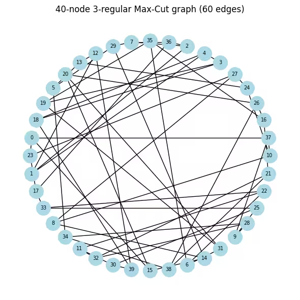
# Visualize the graph so it is clear what problem we are solving before any
# quantum work. Nodes in a circular layout; each edge contributes +1 to the
# cut value when its endpoints land in different partitions.
pos_large = nx.circular_layout(G_large)
fig, ax = plt.subplots(figsize=(6, 6))
nx.draw(
    G_large,
    pos_large,
    with_labels=True,
    node_color="lightblue",
    node_size=400,
    font_size=7,
    ax=ax,
)
ax.set_title(f"40-node 3-regular Max-Cut graph ({len(edges_large)} edges)")
plt.tight_layout()
plt.show()

# Same Maxcut → OptimizationProblem → QUBO → Ising pipeline as the small example,
# applied to the 40-node graph.
prob_large = Maxcut(G_large).to_optimization_problem()
converter_large = OptimizationProblemToQubo()
qubo_large = converter_large.convert(prob_large)
cost_op_large, offset_large = to_ising(qubo_large)
n_qubits_large = cost_op_large.num_qubits
print(
    f"Cost operator: {n_qubits_large} qubits, {len(cost_op_large)} Pauli terms"
)

# ── Step 1b: QP relaxation (multi-start L-BFGS-B) ─────────────────────────
# Same multi-start approach as the small example. At 40 qubits the relaxed
# landscape has many more local minima, so 200 random starts are essential
# to find a low-energy warm-start point.
Q_large = qubo_large.objective.quadratic.to_array(symmetric=True)
mu_large = qubo_large.objective.linear.to_array()

def qp_obj_large(x):
    return x @ Q_large @ x + mu_large @ x + qubo_large.objective.constant

bounds_large = [(0.0, 1.0)] * n_qubits_large
rng_qp = np.random.default_rng(42)
best_val_large, c_star_large = np.inf, None

for _ in range(200):
    x0 = rng_qp.uniform(0.0, 1.0, n_qubits_large)
    res = minimize(qp_obj_large, x0, method="L-BFGS-B", bounds=bounds_large)
    if res.fun < best_val_large:
        best_val_large, c_star_large = res.fun, res.x

# Regularize and convert to rotation angles (same formula as small example)
epsilon_large = 0.25
c_clipped_large = np.clip(c_star_large, epsilon_large, 1 - epsilon_large)
thetas_large = 2 * np.arcsin(np.sqrt(c_clipped_large))
print(
    f"c* range: [{c_star_large.min():.3f}, {c_star_large.max():.3f}]  "
    f"theta range: [{thetas_large.min():.3f}, {thetas_large.max():.3f}] rad"
)

# Plot the distribution of c* values to see how much structure the relaxation
# extracted. Values near 0/1 mean confident assignments; values near 0.5 mean
# the classical solver was uncertain and quantum exploration is most needed there.
fig, ax = plt.subplots(figsize=(6, 3))
ax.hist(c_star_large, bins=20, color="steelblue", edgecolor="white")
ax.axvline(0.5, color="k", linestyle="--", label="Uniform prior (std QAOA)")
ax.set_xlabel(r"$c^*_i$")
ax.set_ylabel("Count")
ax.set_title(r"Distribution of warm-start values $c^*_i$ (40-node graph)")
ax.legend()
plt.tight_layout()
plt.show()

# ── Step 1c: Build WS-QAOA circuit ─────────────────────────────────────────
# Reuse build_ws_qaoa from the small-scale section unchanged; the helper
# scales automatically with n_qubits and the cost operator size.
p_large = 1
ws_qc_large, ws_gammas_large, ws_betas_large = build_ws_qaoa(
    cost_op_large, p_large, n_qubits_large, thetas_large
)
ws_qc_large.measure_all()

# ── Step 2: Transpile to hardware-native gates ──────────────────────────
# generate_preset_pass_manager compiles the abstract circuit to th
# gate set of the backend and inserts SWAP gates wherever the cost Hamiltonian
# couples qubits that are not directly connected on the processor.
pm = generate_preset_pass_manager(optimization_level=3, backend=backend)
ws_isa_large = pm.run(ws_qc_large)

ecr_count = ws_isa_large.count_ops().get("ecr", 0)
print(
    f"\nTranspiled circuit: 2Q depth={ws_isa_large.depth(lambda x: x.operation.num_qubits == 2)}"
)
ws_isa_large.draw("mpl", fold=-1)

Graph: 40 nodes, 60 edges (3-regular)

Cost operator: 40 qubits, 60 Pauli terms
c* range: [0.000, 1.000]  theta range: [1.047, 2.094] rad

Transpiled circuit: 2Q depth=86

# ── Classical baseline via simulated annealing ────────────────────
# Run SA before any hardware calls to get a strong classical reference cut
# value. SA is fast (seconds), needs no solver license, and reliably finds
# near-optimal solutions on 40-node graphs. We use sa_cut as the denominator
# for the approximation ratio instead of the looser QP upper bound.
#
# At each step we flip a random node and accept the move if it improves the
# cut, or with probability exp(delta/T) otherwise. Temperature T decays
# geometrically, allowing uphill moves early on to escape local minima.
def simulated_annealing_maxcut(
    G, seed=0, T0=2.0, T_min=1e-4, alpha=0.995, n_steps=100_000
):
    rng_sa = np.random.default_rng(seed)
    n = G.number_of_nodes()
    x = rng_sa.integers(0, 2, n)
    best_x = x.copy()
    best_cut = sum(1 for u, v in G.edges() if x[u] != x[v])
    T = T0
    for _ in range(n_steps):
        i = rng_sa.integers(0, n)
        delta = sum((-1 if x[i] != x[nb] else 1) for nb in G.neighbors(i))
        if delta > 0 or rng_sa.random() < np.exp(delta / T):
            x[i] ^= 1
            cut = sum(1 for u, v in G.edges() if x[u] != x[v])
            if cut > best_cut:
                best_cut, best_x = cut, x.copy()
        T = max(T * alpha, T_min)
    return best_x, best_cut

sa_solution, sa_cut = simulated_annealing_maxcut(G_large)
print(f"Simulated annealing cut value: {sa_cut}  (classical reference)")

# ── Step 3: Execution on hardware ───────────────────────────
# A Session reserves the backend so the COBYLA iterations and final sampling
# run back-to-back without re-queuing between jobs — important when the
# optimizer submits many short jobs sequentially. All jobs are tagged with
# "TUT_WSQAOA" for traceability in the IBM Quantum dashboard.
#
# EstimatorV2 with resilience_level=1 enables twirled readout error extinction
# (TREX), which corrects systematic measurement bit-flip errors without extra
# circuit overhead. 4096 shots per call balances estimation noise vs. job time.
estimator_options = EstimatorOptions()
estimator_options.resilience_level = 1
estimator_options.default_shots = 4096
estimator_options.environment.job_tags = ["TUT_WSQAOA"]

# Align the cost observable with the physical qubit layout chosen by the transpiler
cost_op_isa = cost_op_large.apply_layout(ws_isa_large.layout)
ws_param_order_isa = list(ws_isa_large.parameters)

ws_history_hw = []

with Session(backend=backend) as session:
    estimator_hw = Estimator(mode=session, options=estimator_options)

    def hw_cost_fn(params):
        bound = ws_isa_large.assign_parameters(
            dict(zip(ws_param_order_isa, params))
        )
        energy = (
            estimator_hw.run([(bound, cost_op_isa)]).result()[0].data.evs.real
        )
        ws_history_hw.append(float(energy))
        print(
            f"  iter {len(ws_history_hw):>3d}  <H_C> = {energy:.4f}", end="\r"
        )
        return float(energy)

    # Warm-start initialization: gamma=0 means the cost unitary is the identity on
    # the first call, so COBYLA immediately evaluates the warm-start state itself —
    # a much better starting signal than a random point.
    ws_params0_hw = np.concatenate(
        [np.zeros(p_large), np.full(p_large, np.pi / 4)]
    )

    ws_result_hw = minimize(
        hw_cost_fn,
        ws_params0_hw,
        method="COBYLA",
        options={"maxiter": 150, "rhobeg": 0.3},
    )
    print(
        f"\nOptimization complete: energy={ws_result_hw.fun:.4f}, "
        f"iterations={len(ws_history_hw)}"
    )

    # ── Step 3b: Sample the optimized circuit ──────────────────────────────────
    # Use 8192 shots for the final sample to get a reliable mode estimate.
    sampler_hw = Sampler(
        mode=session,
        options={"environment": {"job_tags": ["TUT_WSQAOA"]}},
    )
    ws_bound_hw = ws_isa_large.assign_parameters(
        dict(zip(ws_param_order_isa, ws_result_hw.x))
    )
    counts_hw = (
        sampler_hw.run([ws_bound_hw], shots=8192)
        .result()[0]
        .data.meas.get_counts()
    )

best_bs_hw = max(counts_hw, key=counts_hw.get)
best_count = counts_hw[best_bs_hw]
total_shots = sum(counts_hw.values())

# Decode: Qiskit returns bitstrings with qubit 0 at the rightmost position,
# so reversing the string maps character index i to variable x_i.
cut_val_hw, s0_hw, s1_hw = evaluate_cut(best_bs_hw[::-1], G_large)

# Compare against simulated annealing.
# A ratio >= 1.0 means WS-QAOA matched or beat the classical SA solution.
# A ratio close to 1.0 (e.g. > 0.95) shows the quantum result is competitive.
approx_ratio_hw = cut_val_hw / sa_cut
print(
    f"Most-probable bitstring frequency: {best_count}/{total_shots} "
    f"({100*best_count/total_shots:.1f}%)"
)
print(
    f"WS-QAOA cut: {cut_val_hw}  |  SA cut: {sa_cut}  "
    f"|  Approximation ratio vs SA: {approx_ratio_hw:.4f}"
)

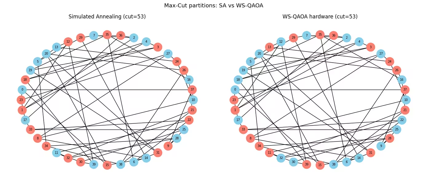
# Visualize both solutions side-by-side on the graph.
# Blue = partition S, orange = partition S-bar.
# Edges crossing between colors are the ones counted in the cut.
fig, axes = plt.subplots(1, 2, figsize=(14, 6))
for ax, assignment, cut, title in [
    (
        axes[0],
        list(sa_solution),
        sa_cut,
        f"Simulated Annealing (cut={sa_cut})",
    ),
    (
        axes[1],
        [int(b) for b in best_bs_hw[::-1]],
        cut_val_hw,
        f"WS-QAOA hardware (cut={cut_val_hw})",
    ),
]:
    colors = [
        "skyblue" if assignment[i] == 0 else "salmon" for i in G_large.nodes()
    ]
    nx.draw(
        G_large,
        pos_large,
        with_labels=True,
        node_color=colors,
        node_size=400,
        font_size=7,
        ax=ax,
    )
    ax.set_title(title)
plt.suptitle("Max-Cut partitions: SA vs WS-QAOA", fontsize=13)
plt.tight_layout()
plt.show()

# ── Step 4: Convergence plot and summary ──────────────────────────────────
# On real hardware the trace will be noisy (shot noise + gate errors), but the
# overall downward trend confirms that COBYLA is making progress despite noise.
fig, ax = plt.subplots(figsize=(7, 4))
ax.plot(ws_history_hw, color="tab:orange", label="WS-QAOA (hardware)")
ax.axhline(
    ws_result_hw.fun,
    color="tab:orange",
    linestyle=":",
    label=f"Final energy ({ws_result_hw.fun:.3f})",
)
ax.set_xlabel("Optimizer call")
ax.set_ylabel(r"$\langle H_C \rangle$")
ax.set_title(f"WS-QAOA convergence on {backend.name} (40 qubits, p=1)")
ax.legend()
plt.tight_layout()
plt.show()

print("\n=== Large Scale Summary ===")
print(f"{'Metric':<38} {'Value':>10}")
print("-" * 50)
print(f"{'Nodes / Edges':<38} {N_LARGE:>5} / {len(edges_large):<4}")
print(f"{'QAOA layers (p)':<38} {p_large:>10}")
print(f"{'Transpiled ECR gate count':<38} {ecr_count:>10}")
print(f"{'Transpiled circuit depth':<38} {ws_isa_large.depth():>10}")
print(f"{'Optimizer iterations':<38} {len(ws_history_hw):>10}")
print(f"{'WS-QAOA energy (hardware)':<38} {ws_result_hw.fun:>10.4f}")
print(f"{'Cut value':<38} {cut_val_hw:>10}")
print(f"{'Simulated annealing cut value':<38} {sa_cut:>10}")
print(f"{'Approximation ratio (vs SA)':<38} {approx_ratio_hw:>10.4f}")

Simulated annealing cut value: 53  (classical reference)
  iter  31  <H_C> = -12.4094
Optimization complete: energy=-13.0256, iterations=31
Most-probable bitstring frequency: 4/8192 (0.0%)
WS-QAOA cut: 53  |  SA cut: 53  |  Approximation ratio vs SA: 1.0000

=== Large Scale Summary ===
Metric                                      Value
--------------------------------------------------
Nodes / Edges                             40 / 60  
QAOA layers (p)                                 1
Transpiled ECR gate count                       0
Transpiled circuit depth                      276
Optimizer iterations                           31
WS-QAOA energy (hardware)                -13.0256
Cut value                                      53
Simulated annealing cut value                  53
Approximation ratio (vs SA)                1.0000

다음 단계

Recommendations

이 작업이 흥미로웠다면 다음 자료에 관심이 있을 수 있습니다:

• 더 높은 QAOA 레이어: p를 늘려 두 알고리즘이 더 많은 회로 레이어와 함께 어떻게 개선되는지, 그리고 낮은 깊이에서의 WS-QAOA 우위가 유지되는지 확인해 보세요.
• Qiskit addon optimization mapper: 문서를 탐색하고 서로 다른 조합 문제를 모델링해 보거나 연속 완화를 위한 다른 솔버를 사용해 보세요.

참고 문헌

[1] D. J. Egger, J. Mareček, and S. Woerner, "Warm-starting quantum optimization," Quantum, vol. 5, p. 479, 2021. arXiv:2009.10095

[2] E. Farhi, J. Goldstone, and S. Gutmann, "A quantum approximate optimization algorithm," arXiv:1411.4028, 2014.