양자 회로로 양자 물질에서 중성자 산란 시뮬레이션하기

사용량 추정치: Heron r2 프로세서에서 13분 (참고: 이는 추정치일 뿐입니다. 실제 실행 시간은 다를 수 있습니다.)

어떤 튜토리얼을 사용해야 할까요?

이 튜토리얼을 사용하면 고전 계산은 노트북에서 로컬로 실행되고 하드웨어 실행은 IBM Quantum® QPU에서 이루어지는 방식으로 구현을 단계별로 배울 수 있어요. 대규모 예제는 상당한 메모리를 필요로 하며, 근사 양자 컴파일링(AQC)은 일반적인 노트북 자원에서 몇 시간이 걸릴 수 있습니다. 압축을 Qiskit Serverless의 컴퓨팅 및 메모리 자원으로 오프로드하려면 함께 제공되는 Serverless 튜토리얼을 사용하세요.

학습 목표

비탄성 중성자 산란(INS) 스펙트럼이 양자 스핀 모델의 동적 구조 인자(DSF)와 어떻게 연결되는지.
바닥 상태를 준비하고, 국소 섭동을 가하며, 양자 회로에서 트로터 시간 전개를 수행하는 방법.
qiskit-addon-aqc-tensor를 사용한 근사 양자 컴파일링(AQC)으로 하드웨어 실행을 위해 깊은 트로터 회로를 압축하는 방법.
큐비트 기댓값으로부터 지연 그린 함수(RGF)를 추출하고 이를 푸리에 변환하여 DSF로 만드는 방법.

필수 조건

배경

이 튜토리얼에서는 Lee 외., arXiv:2603.15608의 결과를 재현합니다.

중성자 산란은 연구자가 배터리 전극을 포함한 지속가능성 관련 소재를 특성화하는 데 도움이 됩니다. 이 튜토리얼은 양자 Circuit이 어떻게 자기 여기를 시뮬레이션하고 이론 모델을 산란 측정과 연결할 수 있는지 탐구합니다. 이 튜토리얼의 양자 자석 예제는 소재 거동을 연구하는 방법을 개발하여 소재 발견을 위한 더 넓은 연구 도구 모음에 기여합니다.

비탄성 중성자 산란과 동적 구조 인자

비탄성 중성자 산란(INS)은 양자 물질에서 자기 여기를 실험적으로 탐구하는 가장 강력한 방법 중 하나입니다. 열 또는 냉 중성자 빔이 결정에 입사하면, 개별 중성자는 자기 서브시스템과 운동량 $\mathbf{q}$ 와 에너지 $\omega$ 를 모두 교환합니다. 측정된 산란 강도는 동적 구조 인자(DSF)에 비례하는데,

$S^{\alpha\beta}(q,\omega) = \sum_{j} e^{-iq\,j}\int_{-\infty}^{\infty} dt\; e^{i\omega t}\, \langle S_0^{\alpha}(0)\, S_j^{\beta}(t)\rangle,$

이는 스핀 자유도의 전체 공간-시간 상관관계를 인코딩합니다.

KCuF $_3$ : 대표적인 러팅거 액체 자성체

불화구리칼륨(KCuF $_3$ )은 스핀- $\frac{1}{2}$ Cu $^{2+}$ 이온 사슬이 최근접 이웃 하이젠베르크 교환 상호작용 $J$ 를 통해 상호작용하는 준1차원 반강자성체이며, 사슬 간 결합은 $J$ 의 $\sim 2.7\%$ 에 불과합니다. INS 데이터가 존재하는 $T = 6\;\mathrm{K}$ 에서, 스펙트럼은 토모나가-러팅거 액체의 특징인 분수화된 스피논 여기가 지배적입니다. 사슬 내 동역학은 등방점( $\epsilon = 1$ )에서의 1차원 스핀- $\frac{1}{2}$ XXZ 해밀토니안으로 잘 기술되므로,

$H = J\sum_{i}\left[S_i^Z S_{i+1}^Z + \epsilon\left(S_i^X S_{i+1}^X + S_i^Y S_{i+1}^Y\right)\right],$

KCuF $_3$ 는 양자 시뮬레이션의 이상적인 벤치마크 역할을 합니다. 해밀토니안은 양자 프로세서에서 구현하기에 충분히 단순하지만, 바닥 상태는 강하게 얽혀 있고 여기 스펙트럼은 넓은 이중-스피논 연속체를 특징으로 합니다.

참고: 이 튜토리얼에서는 $J = 1$ 을 에너지 단위로 설정하고, 논문의 회로 구현(보충 자료 그림 S3)에서 사용된 국소 해밀토니안 $H_\mathrm{loc} = J(S^X S^X + S^Y S^Y + S^Z S^Z)$ 에 해당하는 정규화 $H = J\sum_i[\ldots]$ 를 채택합니다. 논문의 전체 해밀토니안(식 3)은 전체적으로 2배의 추가 계수를 가지므로, 논문의 $J$ 는 여기서 사용된 $J$ 의 두 배입니다.

시뮬레이션 및 측정 대상

우리가 계산하는 물리량은 시간에 따른 스핀-스핀 상관 함수로 정의되는 지연 그린 함수(RGF)입니다.

$G^R_{\alpha,\beta}(j, j_c, t) = -\frac{i}{2}\,\langle\psi_{\mathrm{GS}}|\,S_j^\alpha(t)\,S_{j_c}^\beta(0) - S_{j_c}^\beta(0)\,S_j^\alpha(t)\,|\psi_{\mathrm{GS}}\rangle,$

여기서 $j_c$ 는 기준 사이트(사슬 중심)이고, $S_j^\alpha(t) = e^{iHt}S_j^\alpha e^{-iHt}$ 는 하이젠베르크 묘사의 스핀 연산자입니다. 이 튜토리얼에서는 $zz$ 성분( $\alpha = \beta = z$ )에 초점을 맞춥니다. 양자 컴퓨터에서 RGF는 바닥 상태를 준비하고, $j_c$ 에서 국소 섭동을 가하고, 섭동된 상태를 시간 전개시킨 다음, 각 시간 단계마다 모든 사이트 $j$ 에서 단일 큐비트 기댓값 $\langle\sigma_j^z\rangle$ 을 측정함으로써 얻습니다. 핵심은 각 $\langle\sigma_j^z\rangle$ 이 바닥 상태 자화와의 차이를 준다는 점입니다. 등방적 하이젠베르크 반강자성체는 사이트당 순 자화가 0이기 때문에( $\langle\sigma_j^z\rangle_\mathrm{GS} = 0$ ), 측정된 원시 값이 별도의 뺄셈 없이 바로 $G^R(j, j_c, t)$ 를 제공합니다.

모든 사이트와 시간 단계에 대해 $G^R(j, j_c, t)$ 를 수집하면, 공간과 시간 모두에 대해 푸리에 변환되어 동적 구조 인자 $S(q,\omega)$ 를 생성하는 2차원 데이터셋을 얻게 됩니다. DSF는 INS 실험에서 직접 측정되는 양으로, 각 운동량 $q$ 와 에너지 $\omega$ 에서 어떤 자기 여기가 존재하는지 알려줍니다. 등방적 하이젠베르크 사슬의 경우 정확한 여기 스펙트럼은 이중-스피논 연속체이며, 넓은 산란 강도 밴드의 형태는 양자 시뮬레이션에 대한 엄격한 종단 간 벤치마크 역할을 합니다. 즉 바닥 상태 준비, 섭동, 트로터 시간 전개, 측정 프로토콜을 한 번에 모두 검증하는 것입니다.

양자 시뮬레이션 워크플로

이 워크플로는 INS 이벤트의 물리학을 그대로 반영합니다. (1) $n$ 개의 큐비트에 다체 바닥 상태 $|\psi_{\mathrm{GS}}\rangle$ 를 준비하고, (2) 중성자의 스핀 전달을 모방하기 위해 사슬 중심에서 국소 스핀 반전 섭동 $U_{j_c} = \frac{1}{\sqrt{2}}(I - i\sigma^z_{j_c})$ 를 가하고, (3) 2차 트로터화를 사용하여 이산적인 시간 단계 동안 $H$ 하에서 전개시키고, (4) 각 단계마다 모든 큐비트에서 $\langle\sigma_i^z\rangle$ 을 측정하여 RGF를 얻습니다. 그런 다음 2차원 이산 푸리에 변환을 통해 DSF $S(q,\omega)$ 를 얻습니다.

우리가 매 시간 단계마다 측정하는 관측량은 각 큐비트 $i$ 에 대한 $\sigma_i^z$ 입니다. Qiskit에서는 이를 SparsePauliOp 연산자 목록으로 표현합니다. 각 사이트마다 $n$ -큐비트 항등 연산자 문자열에 하나의 단일 큐비트 $Z$ 를 끼워 넣은 형태입니다. 이러한 관측량은 문제 매핑 단계(1단계)에서 문제 인스턴스당 한 번 구성되며 해당 규모의 모든 회로에서 재사용됩니다.

근사 양자 컴파일링(AQC)

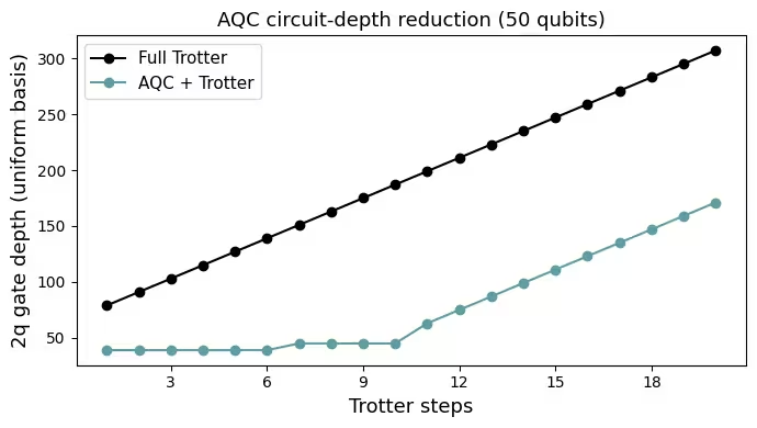
깊은 트로터 회로는 **근사 양자 컴파일링(AQC)**을 통해 압축할 수 있습니다. 이는 처음 몇 개의 트로터 레이어를 더 짧은 매개변수화된 앤자츠로 대체하는 방식이며, 이 앤자츠의 매개변수는 원래의 깊은 회로와의 MPS 수준 충실도를 최대화하도록 고전적으로 최적화됩니다. 나머지 트로터 단계는 정확하게 그대로 추가되어, 2-큐비트 게이트 수가 훨씬 적은 "혼합" AQC + 트로터 회로가 만들어집니다.

MPS 시뮬레이션

1차원 시스템의 경우, 행렬곱상태(MPS) 방법을 사용하면 바닥 상태 준비(밀도 행렬 재규격화군, 즉 DMRG)와 회로 수준의 시간 전개를 모두 효율적으로 시뮬레이션할 수 있습니다. 결합 차원 $\chi$ 를 조절함으로써 정확도와 계산 비용 사이의 균형을 맞출 수 있습니다. 이 튜토리얼에서는 qiskit-addon-aqc-tensor 내에서 MPS 시뮬레이션을 사용하여 하드웨어 실행을 위해 깊은 트로터 회로를 압축하는 고충실도 AQC 앤자츠를 계산합니다.

요구 사항

이 튜토리얼을 시작하기 전에 다음 사항이 설치되어 있는지 확인하세요.

시각화 지원이 포함된 Qiskit SDK
Qiskit Runtime (pip install qiskit-ibm-runtime)
quimb와 JAX 추가 기능이 포함된 qiskit-addon-aqc-tensor (pip install 'qiskit-addon-aqc-tensor[quimb-jax]')

설정

# Added by doQumentation — installs the packages this notebook needs if they are missing
import importlib.util

_needed = {"matplotlib": "matplotlib", "numpy": "numpy", "qiskit": "qiskit", "qiskit_addon_aqc_tensor": "qiskit-addon-aqc-tensor", "qiskit_ibm_runtime": "qiskit-ibm-runtime", "qiskit_quimb": "qiskit-quimb", "quimb": "quimb", "scipy": "scipy"}
_missing = [pip for module, pip in _needed.items()
            if importlib.util.find_spec(module) is None]
# One at a time, so a package that fails to install does not block the others
for _pip in _missing:
    %pip install -q {_pip}
if not _missing:
    print("\u2713 All required packages are installed")

import timeit
import warnings
from collections.abc import Iterator, Sequence
from functools import partial

import matplotlib.pyplot as plt
import numpy as np
import quimb.tensor as qtn
import scipy.optimize
from numpy.typing import NDArray
from qiskit import QuantumCircuit
from qiskit.circuit import CircuitInstruction, ParameterVector, Qubit
from qiskit.circuit.library import PauliEvolutionGate
from qiskit.primitives import StatevectorEstimator
from qiskit.quantum_info import SparsePauliOp
from qiskit.transpiler.preset_passmanagers import generate_preset_pass_manager
from qiskit_addon_aqc_tensor import generate_ansatz_from_circuit
from qiskit_addon_aqc_tensor.objective import MaximizeStateFidelity
from qiskit_addon_aqc_tensor.simulation import tensornetwork_from_circuit
from qiskit_addon_aqc_tensor.simulation.quimb import QuimbSimulator
from qiskit_ibm_runtime import EstimatorV2 as Estimator
from qiskit_ibm_runtime import QiskitRuntimeService
from qiskit_quimb import quimb_circuit
from scipy.sparse import SparseEfficiencyWarning

# scipy.sparse.linalg.expm (reached via PauliEvolutionGate.to_matrix) prefers
# CSC and warns when handed the CSR matrix from SparsePauliOp.to_matrix; the
# result is unaffected, so silence the cosmetic warning.
warnings.filterwarnings("ignore", category=SparseEfficiencyWarning)

def xxz_hamiltonian_mpo(
    n_qubits: int, interaction: float = 1.0, anisotropy: float = 1.0
) -> qtn.MatrixProductOperator:
    """1D XXZ Hamiltonian as a quimb MPO.

    Builds the Hamiltonian using ``qtn.SpinHam1D``.

    Args:
        n_qubits: Number of sites.
        interaction: Overall interaction strength (J in the paper).
        anisotropy: XY/Z anisotropy (ε in the paper). ``ε = 1`` is the
            isotropic Heisenberg point; ``ε = 0`` is the Ising limit.

    Returns:
        The Hamiltonian as a matrix product operator.
    """
    builder = qtn.SpinHam1D(S=1 / 2)
    builder += interaction * anisotropy * 0.5, "+", "-"
    builder += interaction * anisotropy * 0.5, "-", "+"
    builder += interaction, "Z", "Z"
    return builder.build_mpo(L=n_qubits)

def build_ground_state_ansatz(n_qubits: int, n_layers: int) -> QuantumCircuit:
    """Hamiltonian variational ansatz (HVA) circuit for ground-state preparation.

    Starts from a product of singlet pairs and applies alternating
    odd/even layers of parameterized XXZ pair-evolution gates.

    The returned circuit is parameterized: it carries a ``ParameterVector``
    named ``"theta"`` of length ``2 * n_layers`` whose values must be
    assigned (e.g. via ``circuit.assign_parameters``) before simulation.
    Element ``2 * r`` is the odd-layer angle and element ``2 * r + 1`` is the
    even-layer angle of layer ``r``.

    Args:
        n_qubits: Number of qubits (must be even).
        n_layers: Number of HVA layers.

    Returns:
        The parameterized HVA preparation circuit.
    """
    theta = ParameterVector("theta", 2 * n_layers)
    circuit = QuantumCircuit(n_qubits)
    # Initial singlet product state
    for i in range(n_qubits // 2):
        circuit.x(2 * i)
        circuit.x(2 * i + 1)
        circuit.h(2 * i + 1)
        circuit.cx(2 * i + 1, 2 * i)
    # Variational layers: each pair gate is exp(-i theta (XX+YY+ZZ)/2)
    pair_ham = SparsePauliOp(
        ["XX", "YY", "ZZ"], coeffs=[0.5, 0.5, 0.5]
    )  # H_pair (HVA form)
    for r in range(n_layers):
        for i in range(1, (n_qubits + 1) // 2):  # odd layer
            circuit.append(
                PauliEvolutionGate(pair_ham, time=theta[2 * r]),
                [2 * i - 1, 2 * i],
            )
        for i in range(n_qubits // 2):  # even layer
            circuit.append(
                PauliEvolutionGate(pair_ham, time=theta[2 * r + 1]),
                [2 * i, 2 * i + 1],
            )
    return circuit

def optimize_ground_state_ansatz(
    ansatz: QuantumCircuit,
    x0: NDArray[np.floating],
    target_mps: qtn.MatrixProductState,
    *,
    max_bond: int | None = None,
    cutoff: float = 1e-10,
    method: str = "COBYQA",
    options: dict | None = None,
) -> scipy.optimize.OptimizeResult:
    """Optimize HVA parameters by maximizing fidelity with a target MPS.

    The HVA circuit is simulated as a matrix product state with the given
    bond-dimension truncation, and the parameters are optimized to maximize
    the state fidelity ``|<psi_HVA | target_mps>|**2`` with the DMRG ground
    state. Both states are normalized, so the minimized objective is the
    infidelity ``1 - |<psi_HVA | target_mps>|**2``.

    Args:
        ansatz: Parameterized HVA circuit from ``build_ground_state_ansatz``.
            The length of ``x0`` must equal ``ansatz.num_parameters``.
        x0: Initial parameters.
        target_mps: Target MPS (DMRG ground state) to maximize fidelity with.
        max_bond: Maximum MPS bond dimension during gate application.
        cutoff: Singular-value cutoff during gate application.
        method: ``scipy.optimize.minimize`` method.
        options: Options dict forwarded to ``scipy.optimize.minimize``.

    Returns:
        The Scipy OptimizeResult.
    """

    def infidelity(params: NDArray[np.floating]) -> float:
        circuit = ansatz.assign_parameters(params)
        circuit_mps = quimb_circuit(
            circuit.decompose(["PauliEvolution"]),
            quimb_circuit_class=qtn.CircuitMPS,
            max_bond=max_bond,
            cutoff=cutoff,
        )
        return 1 - abs(circuit_mps.psi.H @ target_mps) ** 2

    return scipy.optimize.minimize(
        infidelity, np.asarray(x0), method=method, options=options
    )

def trotter_evolution(
    qubits: Sequence[Qubit],
    interaction: float,
    anisotropy: float,
    time_step: float,
    n_steps: int,
) -> Iterator[CircuitInstruction]:
    """Second-order Trotter steps of the XXZ pair Hamiltonian.

    While the paper used a hand-optimized circuit for the Trotter steps, we use
    PauliEvolutionGate here for simplicity and generality. The final two-qubit gate
    count and gate depth are equivalent when transpiled with ``optimization_level=3``.

    Args:
        qubits: Qubits to act on (length ``n_qubits``).
        interaction: Overall interaction strength (J in the paper).
        anisotropy: XY/Z anisotropy (ε in the paper). ``ε = 1`` is the
            isotropic Heisenberg point; ``ε = 0`` is the Ising limit.
        time_step: Per-step Trotter time.
        n_steps: Number of Trotter steps.

    Yields:
        ``CircuitInstruction``s implementing the Trotter steps.
    """
    if n_steps == 0:
        return
    n_qubits = len(qubits)
    pair_ham = SparsePauliOp(
        ["XX", "YY", "ZZ"],
        coeffs=[
            0.25 * interaction * anisotropy,
            0.25 * interaction * anisotropy,
            0.25 * interaction,
        ],
    )
    half_evo = PauliEvolutionGate(pair_ham, time=time_step / 2)
    full_evo = PauliEvolutionGate(pair_ham, time=time_step)
    for i in range(n_qubits // 2):  # half even layer
        yield CircuitInstruction(half_evo, (qubits[2 * i], qubits[2 * i + 1]))
    for i in range(n_qubits // 2 - 1):  # full odd layer
        yield CircuitInstruction(
            full_evo, (qubits[2 * i + 1], qubits[2 * i + 2])
        )
    for _ in range(n_steps - 1):  # interior steps
        for i in range(n_qubits // 2):
            yield CircuitInstruction(
                full_evo, (qubits[2 * i], qubits[2 * i + 1])
            )
        for i in range(n_qubits // 2 - 1):
            yield CircuitInstruction(
                full_evo, (qubits[2 * i + 1], qubits[2 * i + 2])
            )
    for i in range(n_qubits // 2):  # half even layer
        yield CircuitInstruction(half_evo, (qubits[2 * i], qubits[2 * i + 1]))

def get_dsf(
    n_qubits: int,
    rgf_mat: NDArray[np.floating],
    time_step: float,
    n_steps: int,
    n_points_momentum: int,
    n_points_frequency: int,
) -> NDArray[np.floating]:
    """Compute the dynamical structure factor from the retarded Green's function.

    Uses the center-site approximation and a discrete Fourier transform.
    The result is symmetrized about the momentum axis and clipped to
    non-negative values, ready for plotting.

    Args:
        n_qubits: Number of qubits (sites).
        rgf_mat: RGF matrix of shape ``(n_steps, n_qubits)``.
        time_step: Trotter time-step size.
        n_steps: Number of time steps.
        n_points_momentum: Number of momentum points.
        n_points_frequency: Number of frequency points.

    Returns:
        DSF array of shape ``(n_points_frequency, n_points_momentum)``,
        symmetrized about the momentum axis and clipped to non-negative values.
    """
    max_frequency = np.pi / time_step
    momentum_range = np.linspace(0, 2 * np.pi, n_points_momentum)
    frequency_range = np.linspace(0, max_frequency, n_points_frequency)
    result = np.zeros((frequency_range.shape[0], momentum_range.shape[0]))
    center = n_qubits // 2 - 1
    for iw, w in enumerate(frequency_range):
        exponent = np.exp(1j * w * time_step * np.arange(1, n_steps + 1))
        # S = sigma/2, so two spin operators contribute a factor of (1/2)(1/2) = 1/4.
        rgf_omega = (
            np.dot(rgf_mat.T, exponent) * time_step / 4
        )  # S(omega): time Fourier slice of the Green's function
        for iq, q in enumerate(momentum_range):
            momentum_phases = np.exp(
                -1j * q * np.arange(-center, center + 2, 1)
            )
            result[iw, iq] = np.imag(np.dot(rgf_omega, momentum_phases))
    result = -(result + result[:, ::-1]) / 2
    result = np.clip(result, a_min=0, a_max=None)
    return result

def plot_dsf(
    dsf: NDArray[np.floating],
    time_step: float,
    n_points_momentum: int,
    n_points_frequency: int,
    title: str | None = None,
) -> None:
    """Heat-map of the dynamical structure factor.

    Args:
        dsf: DSF array of shape ``(n_points_frequency, n_points_momentum)``.
        time_step: Trotter time-step size.
        n_points_momentum: Number of momentum points.
        n_points_frequency: Number of frequency points.
        title: Optional plot title.
    """
    max_frequency = np.pi / time_step
    momentum_range = np.linspace(0, 2 * np.pi, n_points_momentum)
    frequency_range = np.linspace(0, max_frequency, n_points_frequency)
    x, y = np.meshgrid(momentum_range, frequency_range)
    fig, ax = plt.subplots(figsize=(8, 5))
    c = ax.pcolormesh(x, y, dsf / np.max(dsf), cmap="viridis", shading="auto")
    fig.colorbar(c, ax=ax, label="Normalized intensity")
    ax.set_ylim(0, 3.6)
    ax.set_xlim(0, 2 * np.pi)
    ax.set_xlabel(r"$q$", fontsize=16)
    ax.set_ylabel(r"$\tilde{\omega} = \omega / J$", fontsize=16)
    ax.set_xticks([0, np.pi / 2, np.pi, 3 * np.pi / 2, 2 * np.pi])
    ax.set_xticklabels(["0", r"$\pi/2$", r"$\pi$", r"$3\pi/2$", r"$2\pi$"])
    if title:
        ax.set_title(title, fontsize=14)
    plt.tight_layout()
    plt.show()

def plot_rgf(
    n_qubits: int,
    rgf_mat: NDArray[np.floating],
    time_step: float,
    n_steps: int,
    title: str | None = None,
) -> None:
    """Heat-map of the retarded Green's function in real space and time.

    Args:
        n_qubits: Number of qubits (sites).
        rgf_mat: RGF matrix of shape ``(n_steps, n_qubits)``.
        time_step: Trotter time-step size.
        n_steps: Number of time steps.
        title: Optional plot title.
    """
    fig, ax = plt.subplots(figsize=(8, 6))
    qubit_axis = np.arange(n_qubits)
    t_axis = np.arange(1, n_steps + 1) * time_step
    x, y = np.meshgrid(qubit_axis, t_axis)
    c = ax.pcolormesh(
        x,
        y,
        np.real(rgf_mat),
        cmap="RdBu",
        vmax=0.5,
        vmin=-0.5,
        shading="auto",
    )
    fig.colorbar(c, ax=ax, label=r"Re $G^R(j, j_c, t)$")
    ax.set_xlabel("Qubit", fontsize=16)
    ax.xaxis.set_major_locator(
        plt.matplotlib.ticker.MaxNLocator(integer=True)
    )
    ax.set_ylabel(r"Time", fontsize=16)
    if title:
        ax.set_title(title, fontsize=14)
    plt.tight_layout()
    plt.show()

def uniform_2q_depth(circuit: QuantumCircuit) -> int:
    """Two-qubit gate depth in a standardized basis."""
    pass_manager = generate_preset_pass_manager(
        optimization_level=0, basis_gates=["cz", "id", "rz", "sx", "x"]
    )
    return pass_manager.run(circuit).depth(
        lambda inst: inst.operation.num_qubits == 2
    )

소규모 시뮬레이터 예제

먼저 MPS 시뮬레이션을 사용하여 HVA 바닥 상태 앤자츠를 최적화하고, 시간 전개를 위해 Qiskit 상태 벡터 시뮬레이터를 사용하여 10 큐비트 규모로 전체 워크플로를 시연합니다. DMRG는 참조 바닥 상태 에너지와 참조 MPS를 제공합니다. 이 소규모 예제를 통해 규모를 확장하기 전에 모든 단계를 검증할 수 있습니다.

1단계: 고전적 입력을 양자 문제로 매핑

먼저 물리적 모델을 정의하고 양자 회로를 구성합니다.

해밀토니안. KCuF $_3$ 는 등방점( $J = 1$ , $\epsilon = 1$ , $J = 1$ 을 에너지 단위로 설정)에서 1차원 XXZ 해밀토니안으로 모델링됩니다.

바닥 상태. 바닥 상태 준비 회로로 해밀토니안 변분 앤자츠(HVA) 회로인 build_ground_state_ansatz를 사용합니다. HVA 매개변수는 DMRG 바닥 상태 MPS와의 상태 충실도 $|\langle\psi_{\mathrm{HVA}}(\theta)|\psi_{\mathrm{DMRG}}\rangle|^2$ 를 최대화함으로써 고전적으로 최적화되며, 이때 HVA 상태는 quimb의 CircuitMPS를 사용하여 회로를 행렬곱상태로 시뮬레이션하여 평가됩니다. 최적화에는 scipy.optimize.minimize를 사용합니다. 참고를 위해 최적화된 앤자츠의 에너지 $\langle H \rangle$ 도 계산됩니다.

트로터 게이트. $H_{\mathrm{pair}} = (J/4)(XX + YY + ZZ)$ 를 갖는 각 최근접 이웃 상호작용 항 $e^{-i\Delta t\, H_{\mathrm{pair}}}$ 는 PauliEvolutionGate(H_pair, time=time_step)로 구성됩니다. Qiskit은 트랜스파일 과정에서 이를 최적의 3-CNOT 분해로 합성합니다.

섭동. 중심 큐비트에 대한 $R_z(\pi/2)$ 게이트는 $U_{j_c} = \frac{1}{\sqrt{2}}(I - i\sigma^z_{j_c})$ 를 구현하여, 산란된 중성자가 발생시키는 국소 스핀 반전을 모방합니다.

관측량. 각 큐비트 사이트에 대해 $\sigma^z$ 관측량을 구성합니다. 이러한 SparsePauliOp 객체는 3단계에서 Estimator 프리미티브에 전달되어 각 시간 단계마다 $\langle\sigma_i^z\rangle$ 를 추출하는 데 사용됩니다.

# -- Physical parameters --
n_qubits = 10
interaction = 1.0  # J
anisotropy = 1.0  # ε (isotropic point)
time_step = 0.6
n_steps = 10
mps_max_bond = 32
mps_cutoff = 1e-8
center = n_qubits // 2 - 1

# -- Hamiltonian MPO --
ham_mpo = xxz_hamiltonian_mpo(n_qubits, interaction, anisotropy)

# -- Reference ground-state energy via DMRG --
dmrg = qtn.DMRG2(ham_mpo)
dmrg.solve(tol=1e-8)
print(f"Ground-state energy (DMRG): {dmrg.energy:.6f}")

# -- Build ground state ansatz circuit --
gs_n_layers = 3
gs_ansatz = build_ground_state_ansatz(n_qubits, gs_n_layers)

# -- Optimize ground state ansatz parameters to maximize fidelity with the DMRG MPS --
# Initialize odd-layer angles near 0 (where the inter-pair gate is the
# identity) and even-layer angles near pi/2 (where the intra-pair gate
# is a SWAP, since 0.5*(XX + YY + ZZ) = SWAP - I/2).
rng = np.random.default_rng(12345)
x0 = np.tile([0, np.pi / 2], gs_n_layers) + rng.normal(
    scale=0.1, size=2 * gs_n_layers
)
print("Optimizing ground state ansatz...")
t0 = timeit.default_timer()
result = optimize_ground_state_ansatz(
    gs_ansatz,
    x0,
    dmrg.state,
    max_bond=mps_max_bond,
    cutoff=mps_cutoff,
    options=dict(maxiter=100),
)
t1 = timeit.default_timer()
print(f"Finished optimizing ground state ansatz in {t1 - t0} seconds.")
print(f"Ground state ansatz fidelity: {1 - result.fun:.6f}")

gs_circuit = gs_ansatz.assign_parameters(result.x)
gs_circuit_mps = quimb_circuit(
    gs_circuit.decompose(["PauliEvolution"]),
    quimb_circuit_class=qtn.CircuitMPS,
    max_bond=mps_max_bond,
    cutoff=mps_cutoff,
)
gs_ansatz_energy = qtn.expec_TN_1D(
    gs_circuit_mps.psi.H, ham_mpo, gs_circuit_mps.psi
)
print(f"Ground state ansatz energy: {gs_ansatz_energy:.6f}")

# -- Build circuits for each time step --
perturbed = gs_circuit.copy()
perturbed.rz(np.pi / 2, center)

circuits = []
for t in range(1, n_steps + 1):
    circuit = perturbed.copy()
    for instr in trotter_evolution(
        circuit.qubits, interaction, anisotropy, time_step, t
    ):
        circuit.append(instr)
    circuits.append(circuit)
print(
    f"Built {len(circuits)} circuits, deepest 2q depth (uniform basis) = "
    f"{uniform_2q_depth(circuits[-1])}"
)

# -- Observables: Z on each qubit site --
observables = [
    SparsePauliOp.from_sparse_list([("Z", [i], 1)], num_qubits=n_qubits)
    for i in range(n_qubits)
]
print(f"Defined {len(observables)} Z observables.")

Ground-state energy (DMRG): -4.258035
Optimizing ground state ansatz...
Finished optimizing ground state ansatz in 8.850687621976249 seconds.
Ground state ansatz fidelity: 0.984277
Ground state ansatz energy: -4.232565
Built 10 circuits, deepest 2q depth (uniform basis) = 163
Defined 10 Z observables.

2단계: 양자 하드웨어 실행을 위한 문제 최적화

실제 하드웨어에서는 위의 트로터 회로가 너무 깊습니다. **근사 양자 컴파일링(AQC)**은 처음 $k$ 개의 트로터 레이어(바닥 상태 회로 포함)를 원래의 깊은 회로와의 MPS 수준 충실도를 최대화하도록 최적화된 더 짧은 매개변수화된 앤자츠로 대체함으로써 이 문제를 해결합니다. 나머지 트로터 단계는 정확하게 그대로 추가되어, 더 얕은 "AQC + 트로터" 회로가 만들어집니다.

표현력과 회로 깊이 사이의 균형을 맞추기 위해 두 가지 앤자츠가 사용됩니다. 단일 트로터 단계로부터 생성되는 1층 앤자츠는 가장 초기의 시간 단계를 압축하고, 두 개의 트로터 단계로부터 생성되는 더 깊은 2층 앤자츠는 더 높은 충실도가 필요한 다음 몇 단계를 압축합니다.

AQC 워크플로에는 네 가지 하위 단계가 있습니다.

목표 회로 구축 — 1단계에서 얻은 처음 $k_1 + k_2$ 개의 회로가 AQC 목표로 직접 사용됩니다.
목표 MPS 계산 — quimb.tensor.CircuitMPS를 사용하여 각 목표 회로를 행렬곱상태로 시뮬레이션합니다.
앤자츠 생성 및 최적화 — generate_ansatz_from_circuit은 1층 및 2층 매개변수화된 앤자츠를 생성합니다. 매개변수는 $1 - |\langle\psi_{\mathrm{ansatz}}|\psi_{\mathrm{target}}\rangle|^2$ 를 최소화하기 위해 JAX 가속 기울기를 사용하는 L-BFGS-B로 최적화됩니다. 처음 $k_1$ 단계는 1층 앤자츠를 사용하고 다음 $k_2$ 단계는 2층 앤자츠를 사용합니다. 각 스테이지 안에서는 직전 시간 단계의 최적화된 매개변수로 워밍스타트하고, 스테이지가 바뀌는 지점에서는 매개변수를 해당 스테이지의 기본값으로 재설정합니다.
혼합 회로 조립 — AQC 체크포인트를 넘어선 시간 단계에 대해 trotter_evolution을 사용하여 최적화된 2층 AQC 회로에 정확한 트로터 레이어를 추가합니다.

# Number of time steps to compress into an AQC ansatz with one layer
aqc_n_steps_1 = 3
# Number of time steps to compress into an AQC ansatz with two layers
aqc_n_steps_2 = 2
aqc_n_steps_total = aqc_n_steps_1 + aqc_n_steps_2

# ── Step 2a: Target circuits (first aqc_n_steps_total circuits from Step 1) ──
target_circuits = {
    k: circuits[k - 1] for k in range(1, aqc_n_steps_total + 1)
}
# ── Step 2b: Compute target MPS ──
# Decompose PauliEvolutionGate to RXX/RYY/RZZ before passing to the AQC MPS
# backend, which does not understand PauliEvolutionGate natively.
aqc_sim = QuimbSimulator(
    quimb_circuit_factory=partial(
        qtn.CircuitMPS,
        gate_opts=dict(max_bond=mps_max_bond, cutoff=mps_cutoff),
    ),
    autodiff_backend="jax",
)
print("\nStep 2b — target MPS:")
target_mps = {}
for k in range(1, aqc_n_steps_total + 1):
    target_mps[k] = tensornetwork_from_circuit(
        target_circuits[k].decompose(["PauliEvolution"]), aqc_sim
    )
    print(f"  k={k}: max bond = {target_mps[k].psi.max_bond()}")

# ── Step 2c: Generate ansätze (one-layer and two-layer) and optimize parameters ──
ansatz_1, initial_params_1 = generate_ansatz_from_circuit(
    target_circuits[1].decompose(["PauliEvolution"]),
    qubits_initially_zero=True,
)
initial_params_1 = np.array(initial_params_1)
ansatz_2, initial_params_2 = generate_ansatz_from_circuit(
    target_circuits[2].decompose(["PauliEvolution"]),
    qubits_initially_zero=True,
)
initial_params_2 = np.array(initial_params_2)
print(
    f"\nStep 2c — one-layer ansatz: {ansatz_1.num_parameters} parameters, "
    f"2q depth (uniform basis) = {uniform_2q_depth(ansatz_1)}"
)
print(
    f"Step 2c — two-layer ansatz: {ansatz_2.num_parameters} parameters, "
    f"2q depth (uniform basis) = {uniform_2q_depth(ansatz_2)}"
)

aqc_circuits = {}
aqc_params = {}
for k in range(1, aqc_n_steps_total + 1):
    if k <= aqc_n_steps_1:
        ansatz, base_params = ansatz_1, initial_params_1
    else:
        ansatz, base_params = ansatz_2, initial_params_2
    # Warm-start from the previous step only within the same stage
    same_stage = (k - 1 >= 1) and (
        (k - 1 <= aqc_n_steps_1) == (k <= aqc_n_steps_1)
    )
    x0 = aqc_params[k - 1] if same_stage else base_params
    obj = MaximizeStateFidelity(target_mps[k], ansatz, aqc_sim)
    t0 = timeit.default_timer()
    result = scipy.optimize.minimize(
        obj.loss_function,
        x0,
        method="L-BFGS-B",
        jac=True,
        options=dict(maxiter=100),
    )
    elapsed = timeit.default_timer() - t0
    aqc_params[k] = result.x
    aqc_circuits[k] = ansatz.assign_parameters(result.x)
    print(
        f"  k={k}: fidelity = {1 - result.fun:.4f}, "
        f"2q depth (uniform basis) = "
        f"{uniform_2q_depth(aqc_circuits[k])}, "
        f"{elapsed:.1f}s"
    )

# ── Step 2d: Assemble full circuit set (AQC + Trotter) ──
all_circuits = []
for k in range(1, aqc_n_steps_total + 1):
    all_circuits.append(aqc_circuits[k])
base = aqc_circuits[aqc_n_steps_total]
for k in range(1, n_steps - aqc_n_steps_total + 1):
    circuit = base.copy()
    for instr in trotter_evolution(
        circuit.qubits, interaction, anisotropy, time_step, k
    ):
        circuit.append(instr)
    all_circuits.append(circuit)

full_depths = [
    uniform_2q_depth(circuits[k - 1]) for k in range(1, n_steps + 1)
]
aqc_depths = [uniform_2q_depth(circuit) for circuit in all_circuits]
full_2q = [
    circuits[k - 1].decompose(["PauliEvolution"]).num_nonlocal_gates()
    for k in range(1, n_steps + 1)
]
aqc_2q = [
    circuit.decompose(["PauliEvolution"]).num_nonlocal_gates()
    for circuit in all_circuits
]
print(f"\nStep 2d — assembled {len(all_circuits)} circuits")
print(
    f"  At step {n_steps} (uniform basis): "
    f"Trotter 2q depth = {full_depths[-1]}, AQC+Trotter 2q depth = {aqc_depths[-1]}; "
    f"2q gates: Trotter = {full_2q[-1]}, AQC+Trotter = {aqc_2q[-1]}"
)

steps_axis = np.arange(1, n_steps + 1)
fig, ax = plt.subplots(figsize=(7, 4))
ax.plot(steps_axis, full_depths, "-o", color="black", label="Full Trotter")
ax.plot(
    steps_axis, aqc_depths, "-o", color="cadetblue", label="AQC + Trotter"
)
ax.set_xlabel("Trotter steps", fontsize=13)
ax.xaxis.set_major_locator(plt.matplotlib.ticker.MaxNLocator(integer=True))
ax.set_ylabel("2q gate depth (uniform basis)", fontsize=13)
ax.set_title(f"AQC circuit-depth reduction ({n_qubits} qubits)", fontsize=13)
ax.legend(fontsize=11)
plt.tight_layout()
plt.show()

Step 2b — target MPS:
  k=1: max bond = 22
  k=2: max bond = 22
  k=3: max bond = 26
  k=4: max bond = 27
  k=5: max bond = 30

Step 2c — one-layer ansatz: 389 parameters, 2q depth (uniform basis) = 27
Step 2c — two-layer ansatz: 470 parameters, 2q depth (uniform basis) = 33
  k=1: fidelity = 1.0000, 2q depth (uniform basis) = 27, 11.8s
  k=2: fidelity = 0.9980, 2q depth (uniform basis) = 27, 13.2s
  k=3: fidelity = 0.9890, 2q depth (uniform basis) = 27, 13.7s
  k=4: fidelity = 0.9983, 2q depth (uniform basis) = 33, 16.4s
  k=5: fidelity = 0.9957, 2q depth (uniform basis) = 33, 16.4s

Step 2d — assembled 10 circuits
  At step 10 (uniform basis): Trotter 2q depth = 163, AQC+Trotter 2q depth = 99; 2q gates: Trotter = 371, AQC+Trotter = 200

Output of the previous code cell

3단계: Qiskit 프리미티브를 사용한 실행

StatevectorEstimator 프리미티브를 사용하여 각 AQC 컴파일 회로를 시뮬레이션합니다.

estimator = StatevectorEstimator()
pubs = [(circuit, observables) for circuit in all_circuits]
job = estimator.run(pubs)
result = job.result()

4단계: 원하는 고전적 형식으로 후처리하고 결과 반환

이제 각 시간 단계 $t$ 에서 모든 큐비트 $i$ 에 대한 기댓값 $\langle\sigma_i^z\rangle$ 을 추출합니다. 이 값들은 지연 그린 함수 행렬 $G^R(j, j_c, t)$ 를 형성합니다. 그런 다음 RGF를 동적 구조 인자 $S(q, \omega)$ 로 푸리에 변환하고 RGF와 DSF를 모두 플로팅합니다. get_dsf는 내부적으로 거울 대칭을 적용하고 음수 값을 잘라냅니다.

rgf_mat = np.stack([pub_result.data.evs for pub_result in result])

# -- Compute DSF --
n_points_momentum, n_points_frequency = 100, 100
spectrum = get_dsf(
    n_qubits,
    rgf_mat,
    time_step,
    n_steps,
    n_points_momentum,
    n_points_frequency,
)

# -- Plot retarded Green's function --
plot_rgf(
    n_qubits,
    rgf_mat,
    time_step,
    n_steps,
    title=f"Retarded Green's function — {n_qubits} qubits (simulation)",
)

# -- Plot DSF --
plot_dsf(
    spectrum,
    time_step,
    n_points_momentum,
    n_points_frequency,
    title=f"Dynamical structure factor — {n_qubits} qubits (simulation)",
)

Output of the previous code cell

대규모 하드웨어 실행

이제 50 큐비트로 규모를 확장합니다. 이 규모에서는 최적화가 소규모 예제보다 낮은 충실도에 도달합니다. 바닥 상태 앤자츠 충실도는 약 0.65로 떨어지고, 이후 체크포인트에서 AQC 충실도는 약 0.7까지 감소합니다. 이는 예상된 결과이며, 바닥 상태 앤자츠 레이어 수(gs_n_layers)나 최적화 반복 횟수(maxiter)를 늘려 추가적인 고전 비용을 들이면 이러한 충실도를 개선할 수 있습니다. 또한 2층 AQC 충실도가 1층보다 낮게 나온다는 점에 유의하세요. 이는 성능 저하가 아닙니다. 이후 시간 단계는 더 많은 얽힘을 생성하여 단순히 압축하기가 더 어렵기 때문이며, 이 때문에 더 표현력이 높은 2층 앤자츠가 사용되는 것입니다.

AQC 최적화에는 몇 시간의 고전 계산 시간이 소요될 수도 있습니다(여기서 보여준 실행에서는 약 6시간이며, 대부분은 2c 단계의 2층 체크포인트에 소요됩니다). 실제 소요 시간을 줄이려면 고성능 컴퓨팅(HPC) 시스템과 같은 더 강력한 고전 하드웨어에서 이 노트북을 실행하는 것을 고려하세요. 또는 더 작은 문제 인스턴스(예: 더 적은 큐비트 수나 더 적은 시간 단계 수)로 규모를 줄일 수도 있으며, 이 경우 결과는 여기서 보여준 것과 달라집니다.

아래 코드는 소규모 예제와 동일한 4단계 구조를 따릅니다. HVA 바닥 상태 매개변수는 다시 MPS 시뮬레이션을 사용하여 최적화됩니다. QPU에서는 오류 억제 및 완화를 위해 동적 디커플링(DD), 파울리 트월링, 트월드 판독 오류 소거(TREX)를 활성화합니다. 다음 표는 대규모 실험이 소규모 실험과 어떻게 다른지를 요약합니다.

	소규모	대규모
큐비트	10	50
시간 단계	10	20
AQC 체크포인트 (1층 + 2층)	3 + 2 = 5	6 + 4 = 10
바닥 상태 앤자츠 레이어	3	5
MPS 최대 결합 차원	32	128
Estimator	`StatevectorEstimator`	DD, 파울리 트월링, TREX를 사용하는 QPU

XLA 느린 컴파일 메시지

AQC 최적화(아래 2c 단계) 중에 다음과 같은 stderr 메시지가 표시될 수 있습니다.

[Compiling module jit_MakeArrayFn for CPU] Very slow compile? ...
The operation took 2m14s

이는 qiskit-addon-aqc-tensor의 JAX 자동미분을 지원하는 컴파일러인 XLA에서 나오는 무해한 진단 메시지입니다. MPS 결합 차원 128을 갖는 50큐비트에서 XLA는 그래디언트 함수를 처음 추적할 때 컴파일에 몇 분을 소요합니다. 컴파일은 성공적으로 완료되며 최적화 결과에는 영향을 미치지 않습니다.

# ── Parameters ──────────────────────────────────────────────────────────────
n_qubits = 50  # 10 → 50
interaction = 1.0  # J
anisotropy = 1.0  # ε (isotropic point)
time_step = 0.6
n_steps = 20  # 10 → 20
aqc_n_steps_1 = 6  # 3 → 6
aqc_n_steps_2 = 4  # 2 → 4
aqc_n_steps_total = aqc_n_steps_1 + aqc_n_steps_2
gs_n_layers = 5  # 3 → 5
mps_max_bond = 128  # 32 -> 128
mps_cutoff = 1e-8
center = n_qubits // 2 - 1

# ── Step 1: Map ──────────────────────────────────────────────────────────────
ham_mpo = xxz_hamiltonian_mpo(n_qubits, interaction, anisotropy)

dmrg = qtn.DMRG2(ham_mpo)
dmrg.solve(tol=1e-8)
print(f"Ground-state energy (DMRG): {dmrg.energy:.6f}")

gs_ansatz = build_ground_state_ansatz(n_qubits, gs_n_layers)

rng = np.random.default_rng(12345)
x0 = np.tile([0.0, np.pi / 2], gs_n_layers) + rng.normal(
    scale=0.1, size=2 * gs_n_layers
)
print("Optimizing ground state ansatz...")
t0 = timeit.default_timer()
result = optimize_ground_state_ansatz(
    gs_ansatz,
    x0,
    dmrg.state,
    max_bond=mps_max_bond,
    cutoff=mps_cutoff,
    options=dict(maxiter=100),
)
t1 = timeit.default_timer()
print(f"Finished optimizing ground state ansatz in {t1 - t0} seconds.")
print(f"Ground state ansatz fidelity: {1 - result.fun:.6f}")

gs_circuit = gs_ansatz.assign_parameters(result.x)
gs_circuit_mps = quimb_circuit(
    gs_circuit.decompose(["PauliEvolution"]),
    quimb_circuit_class=qtn.CircuitMPS,
    max_bond=mps_max_bond,
    cutoff=mps_cutoff,
)
gs_ansatz_energy = qtn.expec_TN_1D(
    gs_circuit_mps.psi.H, ham_mpo, gs_circuit_mps.psi
)
print(f"Ground state ansatz energy: {gs_ansatz_energy:.6f}")

perturbed = gs_circuit.copy()
perturbed.rz(np.pi / 2, center)

circuits = []
for t in range(1, n_steps + 1):
    circuit = perturbed.copy()
    for instr in trotter_evolution(
        circuit.qubits, interaction, anisotropy, time_step, t
    ):
        circuit.append(instr)
    circuits.append(circuit)
print(
    f"Built {len(circuits)} circuits, deepest 2q depth (uniform basis) = "
    f"{uniform_2q_depth(circuits[-1])}"
)

observables = [
    SparsePauliOp.from_sparse_list([("Z", [i], 1)], num_qubits=n_qubits)
    for i in range(n_qubits)
]
print(f"Defined {len(observables)} Z observables.")

# ── Step 2: AQC ──────────────────────────────────────────────────────────────
target_circuits = {
    k: circuits[k - 1] for k in range(1, aqc_n_steps_total + 1)
}

aqc_sim = QuimbSimulator(
    quimb_circuit_factory=partial(
        qtn.CircuitMPS,
        gate_opts=dict(max_bond=mps_max_bond, cutoff=mps_cutoff),
    ),
    autodiff_backend="jax",
)
print("\nStep 2b — target MPS:")
target_mps = {}
for k in range(1, aqc_n_steps_total + 1):
    target_mps[k] = tensornetwork_from_circuit(
        target_circuits[k].decompose(["PauliEvolution"]), aqc_sim
    )
    print(f"  k={k}: max bond = {target_mps[k].psi.max_bond()}")

ansatz_1, initial_params_1 = generate_ansatz_from_circuit(
    target_circuits[1].decompose(["PauliEvolution"]),
    qubits_initially_zero=True,
)
initial_params_1 = np.array(initial_params_1)
ansatz_2, initial_params_2 = generate_ansatz_from_circuit(
    target_circuits[2].decompose(["PauliEvolution"]),
    qubits_initially_zero=True,
)
initial_params_2 = np.array(initial_params_2)
print(
    f"\nStep 2c — one-layer ansatz: {ansatz_1.num_parameters} parameters, "
    f"2q depth (uniform basis) = {uniform_2q_depth(ansatz_1)}"
)
print(
    f"Step 2c — two-layer ansatz: {ansatz_2.num_parameters} parameters, "
    f"2q depth (uniform basis) = {uniform_2q_depth(ansatz_2)}"
)

aqc_circuits = {}
aqc_params = {}
for k in range(1, aqc_n_steps_total + 1):
    if k <= aqc_n_steps_1:
        ansatz, base_params = ansatz_1, initial_params_1
    else:
        ansatz, base_params = ansatz_2, initial_params_2
    # Warm-start from the previous step only within the same stage
    same_stage = (k - 1 >= 1) and (
        (k - 1 <= aqc_n_steps_1) == (k <= aqc_n_steps_1)
    )
    x0 = aqc_params[k - 1] if same_stage else base_params
    obj = MaximizeStateFidelity(target_mps[k], ansatz, aqc_sim)
    t0 = timeit.default_timer()
    result = scipy.optimize.minimize(
        obj.loss_function,
        x0,
        method="L-BFGS-B",
        jac=True,
        options=dict(maxiter=100),
    )
    elapsed = timeit.default_timer() - t0
    aqc_params[k] = result.x
    aqc_circuits[k] = ansatz.assign_parameters(result.x)
    print(
        f"  k={k}: fidelity = {1 - result.fun:.4f}, "
        f"2q depth (uniform basis) = "
        f"{uniform_2q_depth(aqc_circuits[k])}, "
        f"{elapsed:.1f}s"
    )

all_circuits = []
for k in range(1, aqc_n_steps_total + 1):
    all_circuits.append(aqc_circuits[k])
base = aqc_circuits[aqc_n_steps_total]
for k in range(1, n_steps - aqc_n_steps_total + 1):
    circuit = base.copy()
    for instr in trotter_evolution(
        circuit.qubits, interaction, anisotropy, time_step, k
    ):
        circuit.append(instr)
    all_circuits.append(circuit)

full_depths = [
    uniform_2q_depth(circuits[k - 1]) for k in range(1, n_steps + 1)
]
aqc_depths = [uniform_2q_depth(circuit) for circuit in all_circuits]
full_2q = [
    circuits[k - 1].decompose(["PauliEvolution"]).num_nonlocal_gates()
    for k in range(1, n_steps + 1)
]
aqc_2q = [
    circuit.decompose(["PauliEvolution"]).num_nonlocal_gates()
    for circuit in all_circuits
]
print(f"\nStep 2d — assembled {len(all_circuits)} circuits")
print(
    f"  At step {n_steps} (uniform basis): "
    f"Trotter 2q depth = {full_depths[-1]}, AQC+Trotter 2q depth = {aqc_depths[-1]}; "
    f"2q gates: Trotter = {full_2q[-1]}, AQC+Trotter = {aqc_2q[-1]}"
)

steps_axis = np.arange(1, n_steps + 1)
fig, ax = plt.subplots(figsize=(7, 4))
ax.plot(steps_axis, full_depths, "-o", color="black", label="Full Trotter")
ax.plot(
    steps_axis, aqc_depths, "-o", color="cadetblue", label="AQC + Trotter"
)
ax.set_xlabel("Trotter steps", fontsize=13)
ax.xaxis.set_major_locator(plt.matplotlib.ticker.MaxNLocator(integer=True))
ax.set_ylabel("2q gate depth (uniform basis)", fontsize=13)
ax.set_title(f"AQC circuit-depth reduction ({n_qubits} qubits)", fontsize=13)
ax.legend(fontsize=11)
plt.tight_layout()
plt.show()

# ── Step 3: Execute on IBM Quantum hardware ───────────────────────────────────
# (replaces StatevectorEstimator)
service = QiskitRuntimeService()
backend = service.least_busy(
    min_num_qubits=n_qubits,
    operational=True,
    simulator=False,
    filters=lambda x: x.configuration().processor_type["family"] == "Heron",
)
print(f"Backend: {backend.name}")

pm = generate_preset_pass_manager(optimization_level=3, backend=backend)
isa_circuits = pm.run(all_circuits, num_processes=1)
isa_2q_depths = [
    isa_circuit.depth(lambda inst: inst.operation.num_qubits == 2)
    for isa_circuit in isa_circuits
]
print(
    f"Transpiled 2q depth (deepest, ISA on {backend.name}): "
    f"{max(isa_2q_depths)} "
    f"(2q gates: {max(isa_circuit.num_nonlocal_gates() for isa_circuit in isa_circuits)})"
)

estimator = Estimator(backend)
estimator.options.environment.job_tags = ["TUT_SNS"]
estimator.options.dynamical_decoupling.enable = True
estimator.options.dynamical_decoupling.sequence_type = "XY4"
estimator.options.twirling.enable_gates = True
estimator.options.twirling.num_randomizations = 1000
estimator.options.twirling.shots_per_randomization = 128
estimator.options.resilience.measure_mitigation = True
estimator.options.resilience.measure_noise_learning.num_randomizations = 32
estimator.options.resilience.measure_noise_learning.shots_per_randomization = 100

pubs = [
    (
        isa_circuit,
        [obs.apply_layout(isa_circuit.layout) for obs in observables],
    )
    for isa_circuit in isa_circuits
]
job = estimator.run(pubs)
print(f"Job ID: {job.job_id()}")

result = job.result()

# ── Step 4: Post-process ──────────────────────────────────────────────────────
rgf_mat = np.stack([pub_result.data.evs for pub_result in result])

n_points_momentum, n_points_frequency = 100, 100
spectrum = get_dsf(
    n_qubits,
    rgf_mat,
    time_step,
    n_steps,
    n_points_momentum,
    n_points_frequency,
)

plot_rgf(
    n_qubits,
    rgf_mat,
    time_step,
    n_steps,
    title=f"Retarded Green's function — {n_qubits} qubits (QPU)",
)
plot_dsf(
    spectrum,
    time_step,
    n_points_momentum,
    n_points_frequency,
    title=rf"KCuF$_3$ DSF — {n_qubits} qubits (QPU)"
    "\n(AQC + DD + Pauli twirling + TREX)",
)

Ground-state energy (DMRG): -21.972109
Optimizing ground state ansatz...
Finished optimizing ground state ansatz in 132.2076231740648 seconds.
Ground state ansatz fidelity: 0.645956
Ground state ansatz energy: -21.616744
Built 20 circuits, deepest 2q depth (uniform basis) = 307
Defined 50 Z observables.

Step 2b — target MPS:
  k=1: max bond = 44
  k=2: max bond = 46
  k=3: max bond = 53
  k=4: max bond = 62
  k=5: max bond = 75
  k=6: max bond = 96
  k=7: max bond = 118
  k=8: max bond = 128
  k=9: max bond = 128
  k=10: max bond = 128

Step 2c — one-layer ansatz: 2971 parameters, 2q depth (uniform basis) = 39
Step 2c — two-layer ansatz: 3412 parameters, 2q depth (uniform basis) = 45
  k=1: fidelity = 1.0000, 2q depth (uniform basis) = 39, 215.6s
  k=2: fidelity = 0.9676, 2q depth (uniform basis) = 39, 269.8s
  k=3: fidelity = 0.9014, 2q depth (uniform basis) = 39, 293.5s
  k=4: fidelity = 0.8755, 2q depth (uniform basis) = 39, 279.6s
  k=5: fidelity = 0.8450, 2q depth (uniform basis) = 39, 266.4s
  k=6: fidelity = 0.8146, 2q depth (uniform basis) = 39, 371.0s

E0626 02:59:07.229070 1508496 slow_operation_alarm.cc:73] 
********************************
[Compiling module jit_MakeArrayFn for CPU] Very slow compile? If you want to file a bug, run with envvar XLA_FLAGS=--xla_dump_to=/tmp/foo and attach the results.
********************************
E0626 02:59:21.713796 1508477 slow_operation_alarm.cc:140] The operation took 2m14.484932074s

********************************
[Compiling module jit_MakeArrayFn for CPU] Very slow compile? If you want to file a bug, run with envvar XLA_FLAGS=--xla_dump_to=/tmp/foo and attach the results.
********************************

k=7: fidelity = 0.7312, 2q depth (uniform basis) = 45, 10865.3s
  k=8: fidelity = 0.7720, 2q depth (uniform basis) = 45, 1450.3s
  k=9: fidelity = 0.7316, 2q depth (uniform basis) = 45, 3388.6s

E0626 07:21:05.148724 1508496 slow_operation_alarm.cc:73] 
********************************
[Compiling module jit_MakeArrayFn for CPU] Very slow compile? If you want to file a bug, run with envvar XLA_FLAGS=--xla_dump_to=/tmp/foo and attach the results.
********************************
E0626 07:21:24.286095 1508477 slow_operation_alarm.cc:140] The operation took 2m19.137566498s

********************************
[Compiling module jit_MakeArrayFn for CPU] Very slow compile? If you want to file a bug, run with envvar XLA_FLAGS=--xla_dump_to=/tmp/foo and attach the results.
********************************

k=10: fidelity = 0.6726, 2q depth (uniform basis) = 45, 3396.1s

Step 2d — assembled 20 circuits
  At step 20 (uniform basis): Trotter 2q depth = 307, AQC+Trotter 2q depth = 171; 2q gates: Trotter = 3775, AQC+Trotter = 1913

Output of the previous code cell

Backend: ibm_fez
Transpiled 2q depth (deepest, ISA on ibm_fez): 105 (2q gates: 2574)
Job ID: d8v39vhropqc738biotg

Output of the previous code cell

하드웨어 결과는 이중-스피논 연속체의 핵심 특징을 재현합니다. 산란 강도는 낮은 에너지에서 반강자성 파동 벡터 $q = \pi$ 근처에 집중되어 있으며, 정현파 모양의 스피논 분산이 하한을 이루고, 단일 날카로운 모드가 아닌 그 위에 넓은 스펙트럼 가중치의 연속체가 존재합니다. 이는 KCuF $_3$ 에 대한 비탄성 중성자 산란으로 측정되는 것과 동일한 구조이며, 50큐비트 규모에서 바닥 상태 준비, 섭동, AQC로 압축된 트로터 전개, 오류 완화 측정의 전체 워크플로를 검증합니다.

다음 단계

이 작업이 흥미로웠다면 다음 자료에 관심이 있을 수 있습니다.

권장 사항

AQC + 트로터 동역학 서버리스 워크플로로 중성자 산란 시뮬레이션하기 — 배포된 Qiskit 서버리스 함수 템플릿을 통해 동일한 실험을 실행하는 동반 튜토리얼
Lee 외, "중성자 산란 실험을 이용한 양자 시뮬레이션 벤치마킹" (arXiv:2603.15608) — 이 튜토리얼이 기반으로 하는 참고 논문
오류 완화 및 억제 기법 — 하드웨어 실험에서 사용된 DD, 파울리 트월링, TREX
시간 전개 회로를 위한 근사 양자 컴파일 — AQC-Tensor에 관한 튜토리얼
AQC-Tensor 문서

학습 목표​

필수 조건​

배경​

비탄성 중성자 산란과 동적 구조 인자​

KCuF3_33​: 대표적인 러팅거 액체 자성체​

시뮬레이션 및 측정 대상​

양자 시뮬레이션 워크플로​

근사 양자 컴파일링(AQC)​

MPS 시뮬레이션​

요구 사항​

설정​

소규모 시뮬레이터 예제​

1단계: 고전적 입력을 양자 문제로 매핑​

2단계: 양자 하드웨어 실행을 위한 문제 최적화​

3단계: Qiskit 프리미티브를 사용한 실행​

4단계: 원하는 고전적 형식으로 후처리하고 결과 반환​

대규모 하드웨어 실행​

다음 단계​

학습 목표

필수 조건

배경

비탄성 중성자 산란과 동적 구조 인자

KCuF $_3$ : 대표적인 러팅거 액체 자성체

시뮬레이션 및 측정 대상

양자 시뮬레이션 워크플로

근사 양자 컴파일링(AQC)

MPS 시뮬레이션

요구 사항

설정

소규모 시뮬레이터 예제

1단계: 고전적 입력을 양자 문제로 매핑

2단계: 양자 하드웨어 실행을 위한 문제 최적화

3단계: Qiskit 프리미티브를 사용한 실행

4단계: 원하는 고전적 형식으로 후처리하고 결과 반환

대규모 하드웨어 실행

다음 단계