AQC + Trotter 동역학 Serverless 워크플로로 중성자 산란 시뮬레이션하기
사용량 추정치: Heron r3 프로세서에서 18분 (참고: 이는 추정치일 뿐입니다. 실제 실행 시간은 다를 수 있습니다.)
학습 목표
-
비탄성 중성자 산란 스펙트럼이 1차원 양자 자석의 동적 구조 인자 에 어떻게 매핑되는지.
-
밀도 행렬 재규격화 그룹(DMRG)과 행렬 곱 상태(MPS) 충실도 최대화를 사용하여 KCuF(등방성 하이젠베르크) 바닥 상태를 준비하는 방법.
-
단일 함수 호출로 Trotter 시간 진화, 근사 양자 컴파일(AQC) 회로 압축, 그리고 오류 완화 실행을 실행하는 방법.
-
사이트별 시계열을 후처리하여 로 변환하고 이중 스피논 연속체를 식별하는 방법.
필수 조건
-
Qiskit 패턴,
SparsePauliOp, 그리고 Trotter 시간 진화에 익숙해지기. -
텐서 네트워크 기법(DMRG, MPS)을 접해본 경험이 있으면 도움이 되지만 필수는 아니며, 이 함수가 Trotter 회로를 압축하는 데 사용하는
qiskit-addon-aqc-tensor라이브러리에 대한 익숙함도 마찬가지입니다.
배경
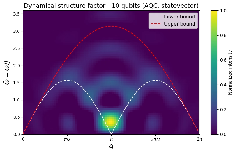
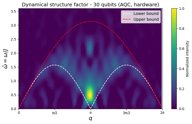
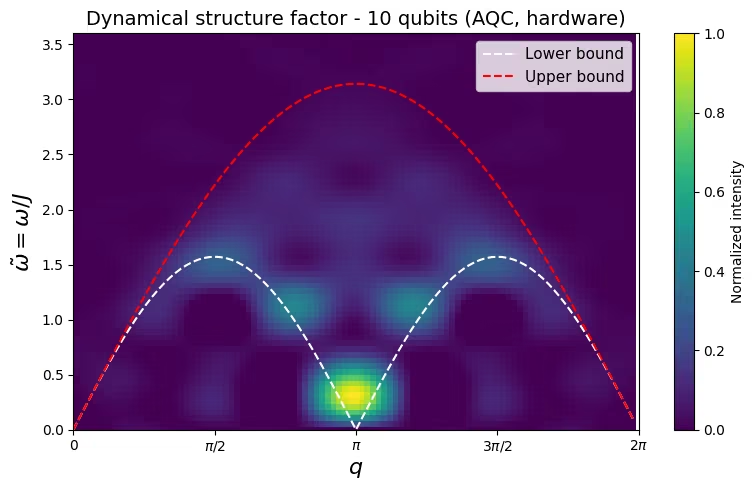
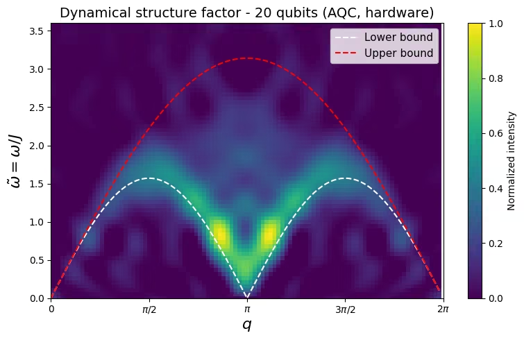
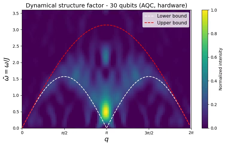
비탄성 중성자 산란은 스핀-스핀 상관 함수의 공간-시간 푸리에 변환인 동적 구조 인자 를 측정하므로, 미시적 스핀 모델로부터 를 재현하는 것은 양자 시뮬레이션에 대한 직접적이고 반증 가능한 테스트입니다. 이 튜토리얼은 스핀- 반강자성 하이젠베르크 사슬인 KCuF를 다루는데, 이 물질의 여기는 단일 스핀 플립이 아니라 쌍의 분수화된 스피논입니다: 날카로운 마그논 분산 대신, 는 아래로는 , 위로는 로 경계 지어진 넓은 이중 스피논 연속체를 보여줍니다. 이는 다음에 나오는 그래프의 점선 곡선입니다. 물리학의 전체 내용과 측정된 중성자 데이터와의 비교는 원본 튜토리얼과 Lee 외., arXiv:2603.15608에서 다룹니다.
양자 워크플로는 산란 실험을 반영합니다:
-
사슬의 바닥 상태 를 준비합니다.
-
중앙 사이트에서 국소적인 교란, 즉 -회전으로 자극하여 중성자로부터의 운동량 및 에너지 전달을 모방합니다.
-
Trotter 곱 공식을 사용하여 하이젠베르크 해밀토니안 하에서 시간 진화합니다.
-
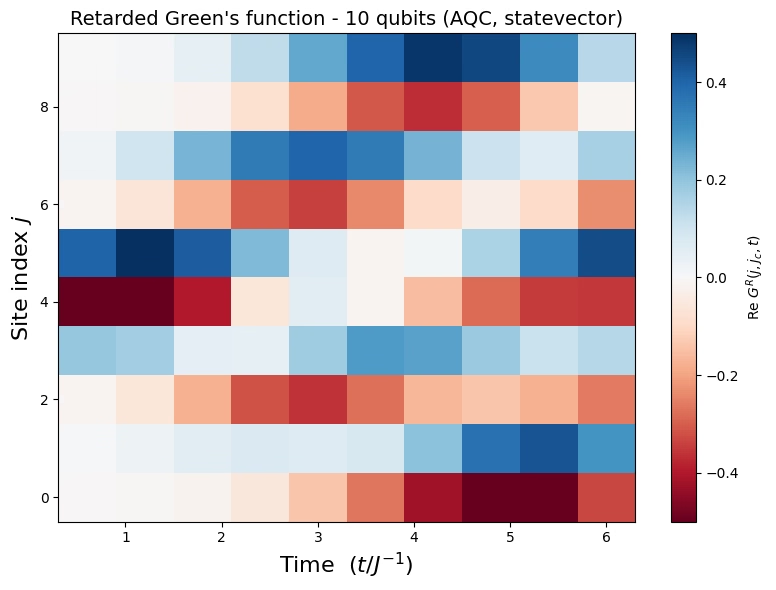
사이트별 자화 를 측정합니다. 사이트 와 시간 의 함수로서 이는 정확히 지연 그린 함수 이므로, 5단계의 푸리에 변환 전에 변환이 필요하지 않습니다.
-
을 푸리에 변환하여 로 만듭니다.
3단계에서 문제가 발생할 수 있는데, 이는 긴 진화에 대한 정확한 Trotter 회로가 하드웨어에서 실행하기에 너무 깊어질 때입니다. 텐서 네트워크를 사용한 AQC는 Trotter 단계의 블록을 고정된 얕은 매개변수화된 앤사츠로 압축함으로써 이 문제를 해결하는데, 이 앤사츠의 정확한 진화에 대한 상태 충실도는 MPS 시뮬레이터를 사용하여 고전적으로 최대화됩니다(arXiv:2301.08609). AQC Dynamics Template은 이 전체 양자 코어(Trotter 합성, AQC 압축, 오류 완화 실행)를 하나의 호출 뒤에 패키징합니다:
| PRE (이 노트북) | FUNCTION (aqc-dynamics-function) | POST (이 노트북) |
|---|---|---|
| DMRG와 MPS 충실도 최대화로부터의 바닥 상태, 중성자 킥이 동일한 회로에 내장됨 | Trotter 합성 → AQC 압축 → statevector, fake, 또는 runtime에서의 실행, 사이트별 반환 | , 동적 구조 인자 |
실험별 작업은 이 노트북에 그대로 남아 있습니다: 바닥 상태 준비(PRE)와 후처리(POST). 양자 연산이 많이 필요한 두 단계인 압축과 실행은 함수 내부에서 실행됩니다.
이 튜토리얼은 동일한 실험을 인라인으로 구축하는 양자 회로로 양자 물질에서 중성자 산란 시뮬레이션하기의 동반 자료입니다: 동일한 KCuF 모델, 바닥 상태 준비, 중성자 킥, 후처리를 다루지만, Trotter 합성, AQC 압축, 오류 완화 실행이 단계별로 작성되어 있습니다. AQC 압축의 작동 방식을 알아보려면 그 튜토리얼을 읽으세요. 배포된 함수 템플릿을 통해 동일한 실험을 실행하려면 이 튜토리얼을 읽으세요: 양자 코어가 단일 함수 호출이 되며, 몇 시간이 걸리는 AQC 압축은 사용자의 컴퓨터가 아닌 Serverless 워커 내부에서 실행되므로 실행되는 동안 HPC 시스템이나 열려 있는 커널이 필요하지 않습니다. 동일한 호출은 다른 1차원 동역학 실험도 구동합니다.
요구 사항
이 튜토리얼을 시작하기 전에 다음 사항을 확인하세요:
-
Qiskit Serverless 계정에 배포된 함수. 먼저 동반 함수 템플릿을 실행하세요: AQC + Trotter 동역학 함수 템플릿 배포 및 실행. 그 가이드는 소스 파일을 가져와서 계정에 함수를 업로드하는 과정을 안내합니다. 이 튜토리얼은 배포된 함수만 호출합니다.
-
QiskitServerless에 저장된 IBM Quantum® 자격 증명(함수 템플릿 참조). 이 튜토리얼의 두 예제 모두 배포된 함수를 호출하므로 둘 다 필요합니다. -
Qiskit SDK v2.0 이상 (
pip install qiskit). -
Qiskit IBM Catalog 클라이언트 (
pip install qiskit-ibm-catalog). -
NumPy, SciPy, Matplotlib (
pip install numpy scipy matplotlib). 바닥 상태 준비에 사용되는 COBYQA 최적화기를 위해 SciPy 1.14 이상이 필요합니다. -
1단계의 바닥 상태 준비가 이 노트북에서 로컬로 실행되므로 AQC 텐서 네트워크 스택:
pip install 'qiskit-addon-aqc-tensor[quimb-jax]==0.3.1'.
새로 배포된 함수에 대한 첫 번째 호출은 Serverless 워커가 종속성을 설치하는 동안 대기하므로, 해당 실행에서 추가 지연이 예상됩니다.
설정
라이브러리를 가져오고 나중에 사용할 실험별 헬퍼를 정의합니다: build_gs_ansatz(바닥 상태 준비를 위한 해밀토니안 변분 앤사츠, 즉 HVA), prepare_ground_state(DMRG와 MPS 충실도 최대화), 그리고 get_spectrum, plot_green, plot_spectrum( 후처리). 이들은 원본 중성자 산란 튜토리얼에서 가져온 것입니다.
# Added by doQumentation — required packages for this notebook
!pip install -q matplotlib numpy qiskit qiskit-addon-aqc-tensor qiskit-ibm-catalog quimb scipy
from functools import partial

import matplotlib.pyplot as plt
import numpy as np
import scipy.optimize

import quimb.tensor as qtn
from qiskit import QuantumCircuit
from qiskit.quantum_info import SparsePauliOp
from qiskit_addon_aqc_tensor.simulation import tensornetwork_from_circuit
from qiskit_addon_aqc_tensor.simulation.quimb import QuimbSimulator
from qiskit_ibm_catalog import QiskitServerless
#  Dynamical structure factor via discrete Fourier transform

def get_spectrum(n, Gjjc, dt, time_steps, q_steps, w_steps):
    """Compute the dynamical structure factor from the retarded Green's function.

    Uses the center-site approximation and a discrete Fourier transform.
    """
    green = Gjjc / 4  # sigma -> S=1/2
    omega_max = np.pi / dt
    qpoints = np.arange(0, 2 * np.pi, 2 * np.pi / q_steps)
    omegas = np.arange(0, omega_max, omega_max / w_steps)
    green_map = np.zeros((omegas.shape[0], qpoints.shape[0]))
    center = n // 2 - 1
    for iw, w in enumerate(omegas):
        exponent = np.exp(1j * w * dt * np.arange(1, time_steps + 1))
        S_w = np.dot(green.T, exponent) * dt
        for iq, q in enumerate(qpoints):
            q_matrix = np.exp(-1j * q * np.arange(-center, center + 2, 1))
            green_map[iw, iq] = np.imag(np.dot(S_w, q_matrix))
    return green_map

#  Plotting helpers

def plot_spectrum(
    dsf,
    dt,
    q_steps,
    w_steps,
    lower_bound=False,
    upper_bound=False,
    title=None,
):
    """Heat-map of the dynamical structure factor."""
    omega_max = np.pi / dt
    qpoints = np.arange(0, 2 * np.pi, 2 * np.pi / q_steps)
    omegas = np.arange(0, omega_max, omega_max / w_steps)
    x, y = np.meshgrid(qpoints, omegas)
    fig, ax = plt.subplots(figsize=(8, 5))
    c = ax.pcolormesh(x, y, dsf / np.max(dsf), cmap="viridis", shading="auto")
    fig.colorbar(c, ax=ax, label="Normalized intensity")
    if lower_bound:
        ax.plot(
            qpoints,
            np.pi * np.abs(np.sin(qpoints)) / 2,
            "--",
            color="white",
            lw=1.5,
            label="Lower bound",
        )
    if upper_bound:
        ax.plot(
            qpoints,
            np.pi * np.abs(np.sin(qpoints / 2)),
            "--",
            color="red",
            lw=1.5,
            label="Upper bound",
        )
    ax.set_ylim(0, 3.6)
    ax.set_xlim(0, 2 * np.pi - 2 * np.pi / q_steps)
    ax.set_xlabel(r"$q$", fontsize=16)
    ax.set_ylabel(r"$\tilde{\omega} = \omega / J$", fontsize=16)
    ax.set_xticks([0, np.pi / 2, np.pi, 3 * np.pi / 2, 2 * np.pi])
    ax.set_xticklabels(["0", r"$\pi/2$", r"$\pi$", r"$3\pi/2$", r"$2\pi$"])
    if lower_bound or upper_bound:
        ax.legend(loc="upper right", fontsize=11)
    if title:
        ax.set_title(title, fontsize=14)
    plt.tight_layout()
    plt.show()

def plot_green(n, Gjjc, time_steps, dt, title=None):
    """Heat-map of the retarded Green's function in real space and time."""
    fig, ax = plt.subplots(figsize=(8, 6))
    t_axis = np.arange(1, time_steps + 1) * dt
    site_axis = np.arange(n)
    x, y = np.meshgrid(t_axis, site_axis)
    c = ax.pcolormesh(
        x,
        y,
        np.real(Gjjc).T,
        cmap="RdBu",
        vmax=0.5,
        vmin=-0.5,
        shading="auto",
    )
    fig.colorbar(c, ax=ax, label=r"Re $G^R(j, j_c, t)$")
    ax.set_xlabel(r"Time  ($t / J^{-1}$)", fontsize=16)
    ax.set_ylabel("Site index $j$", fontsize=16)
    if title:
        ax.set_title(title, fontsize=14)
    plt.tight_layout()
    plt.show()

#  Variational ground-state ansatz (HVA)

def _apply_xxz_pair_gate(qc, q0, q1, theta):
    """Apply the parameterized XXZ-type two-qubit gate used in the HVA."""
    qc.cx(q0, q1)
    qc.rz(theta, q1)
    qc.h(q0)
    qc.rz(theta + np.pi / 2, q0)
    qc.cx(q0, q1)
    qc.rz(-theta, q1)
    qc.h(q1)
    qc.cx(q1, q0)
    qc.rz(np.pi / 2, q1)
    qc.rz(-np.pi / 2, q0)
    qc.h(q1)
    qc.h(q0)

def build_gs_ansatz(n, params, layers):
    """Build the Hamiltonian variational ansatz (HVA) circuit for
    ground-state preparation of the 1D Heisenberg model.

    Starts from a product of singlet pairs and applies alternating
    odd/even layers of parameterized XXZ gates. For layer r,
    params[2 * r] is the odd-layer (inter-pair) angle and
    params[2 * r + 1] is the even-layer (intra-pair) angle.
    """
    qc = QuantumCircuit(n)
    # Initial singlet product state
    for i in range(n // 2):
        qc.x(2 * i)
        qc.x(2 * i + 1)
        qc.h(2 * i + 1)
        qc.cx(2 * i + 1, 2 * i)
    # Variational layers
    for r in range(layers):
        for i in range(1, (n + 1) // 2):  # odd layer
            _apply_xxz_pair_gate(qc, 2 * i - 1, 2 * i, params[2 * r])
        for i in range(n // 2):  # even layer
            _apply_xxz_pair_gate(qc, 2 * i, 2 * i + 1, params[2 * r + 1])
    return qc

def prepare_ground_state(n, gs_layers=5, max_bond=128, cutoff=1e-8):
    """Prepare the KCuF3 (isotropic Heisenberg) ground state as a QuantumCircuit.

    Runs DMRG (quimb MPO + DMRG2) to get the chain's ground state, then optimizes
    the HVA angles to maximize the MPS overlap |<psi_ansatz|psi_DMRG>|^2. No exact
    diagonalization, so it scales to larger n.
    """
    J = Jz = 1.0
    builder = qtn.SpinHam1D(S=1 / 2)
    builder += J * 0.5, "+", "-"
    builder += J * 0.5, "-", "+"
    builder += Jz, "Z", "Z"
    H_mpo = builder.build_mpo(L=n)
    dmrg = qtn.DMRG2(H_mpo)
    dmrg.solve(tol=1e-8, verbosity=0)

    gs_sim = QuimbSimulator(
        quimb_circuit_factory=partial(
            qtn.CircuitMPS, gate_opts=dict(cutoff=cutoff, max_bond=max_bond)
        ),
        autodiff_backend="jax",
    )

    def gs_infidelity(params):
        psi = tensornetwork_from_circuit(
            build_gs_ansatz(n, params, gs_layers), gs_sim
        ).psi
        return 1 - abs(psi.H @ dmrg.state) ** 2

    # Seed and optimizer match the original tutorial. Each layer starts at
    # [0, pi/2]: an odd-layer angle of 0 makes the inter-pair gate the identity,
    # and an even-layer angle of pi/2 makes the intra-pair gate a SWAP (since
    # 0.5 * (XX + YY + ZZ) = SWAP - I/2). That puts the seed at the singlet-pair
    # product limit, which is already a decent approximation to the Heisenberg
    # ground state, so the optimizer only has to refine it. The small jitter
    # (fixed RNG seed, so runs are reproducible) breaks the exact symmetry
    # between layers; COBYQA then runs for up to 100 iterations.
    rng = np.random.default_rng(12345)
    x0 = np.tile([0.0, np.pi / 2], gs_layers) + rng.normal(
        scale=0.1, size=2 * gs_layers
    )
    result_gs = scipy.optimize.minimize(
        gs_infidelity, x0, method="COBYQA", options={"maxiter": 100}
    )
    print(f"DMRG ground-state energy: {dmrg.energy:.6f}")
    print(f"GS fidelity: {1 - result_gs.fun:.4f}")
    return build_gs_ansatz(n, result_gs.x, gs_layers)

print("Setup complete - helpers defined.")
Setup complete - helpers defined.
함수 템플릿 로드하기
Qiskit Serverless에 연결하고 배포된 aqc-dynamics-function을 로드합니다. 이 튜토리얼의 두 예제 모두 동일한 fn 핸들을 호출하므로, 함수는 여기서 한 번만 로드됩니다.
# Credentials are read from the account saved once via QiskitServerless.save_account(...)
serverless = QiskitServerless()
fn = serverless.load("aqc-dynamics-function")
소규모 시뮬레이터 예제
먼저 정확한 statevector 백엔드를 사용하여 작은 10사이트 사슬에서 전체 워크플로를 실행합니다. 이는 QPU 시간을 소비하기 전에 PRE → FUNCTION → POST 파이프라인을 검증합니다.
1단계: 고전적 입력을 양자 문제로 매핑하기
KCuF 해밀토니안을 SparsePauliOp로 구축합니다(등방성 하이젠베르크: 각 최근접 이웃 결합에서 결합 상수 의 ; 문자열은 Pauli 연산자이므로 는 스핀- 결합을 제공합니다). DMRG와 MPS 충실도 최대화로 바닥 상태를 준비한 다음, 중앙 사이트에서 -회전인 중성자 킥을 내장합니다. 준비된 회로는 initial_state로 함수에 전달하는 것입니다. observables는 기본값(사이트별 )으로 그대로 두는데, 이는 중성자 워크플로에 필요한 정확한 판독값입니다.
n = 10
dt = 0.6  # physical time per Trotter step (also the omega-axis unit in POST)
time_steps = 10
center = n // 2 - 1

# MPS-simulator settings, shared by the ground-state prep here and the AQC
# compression inside the function (matches the original tutorial).
mps_max_bond = 32
mps_cutoff = 1e-8

# 1D isotropic Heisenberg (KCuF3) Hamiltonian on n qubits
H = SparsePauliOp.from_sparse_list(
    [(p, [i, i + 1], 0.25) for i in range(n - 1) for p in ("XX", "YY", "ZZ")],
    num_qubits=n,
)

# Ground state (DMRG + fidelity max) + neutron kick baked into the same circuit
gs_circuit = prepare_ground_state(
    n, gs_layers=3, max_bond=mps_max_bond, cutoff=mps_cutoff
)
gs_circuit.rz(
    np.pi / 2, center
)  # exp(-i (pi/2)/2 Z_center): the neutron perturbation
print(
    f"Prepared {n}-qubit ground state with the neutron kick at site {center}."
)
DMRG ground-state energy: -4.258035
GS fidelity: 0.9841
Prepared 10-qubit ground state with the neutron kick at site 4.
2단계와 3단계: 함수 템플릿으로 압축 및 실행하기
수작업 워크플로에서는 이것들이 두 개의 별도 단계입니다: 하드웨어용으로 회로를 최적화하기(2단계)와 실행하기(3단계). 함수 템플릿은 두 단계를 하나의 호출로 축소합니다. Trotter 합성, AQC 압축, 하드웨어 트랜스파일을 수행한 다음 회로를 실행합니다(여기서는 정확한 시뮬레이터에서, 나중에는 하드웨어에서 내장된 오류 완화 기능과 함께). 두 개의 조정 매개변수는 aqc_segments(압축 계획)와 aqc_options(MPS 및 최적화기 설정)입니다. 각 세그먼트 {"n_steps": k, "ansatz_steps": m}는 k개의 연속된 Trotter 단계를 m단계 Trotter 대상으로 구축된 앤사츠로 압축하며, sum(n_steps)를 넘어서는 단계는 일반 Trotter로 실행됩니다. 초기의, 엉킴이 적은 단계는 얕은(ansatz_steps=1) 앤사츠로 잘 압축되므로, 여기서는 처음 세 단계를 단일 계층 앤사츠로, 다음 두 단계를 더 깊은 이중 계층 앤사츠로 압축하고, 10개의 Trotter 단계 중 나머지 다섯 개는 일반 Trotter로 실행합니다. aqc_options의 경우 원본 튜토리얼을 반영합니다: MPS 결합 차원 max_bond=32, cutoff=1e-8, 그리고 100회로 제한된 L-BFGS-B 최적화기.
설정에서 로드된 함수를 호출합니다. backend="statevector"는 정확한 참조 경로를 실행합니다: QPU 시간이 소요되지 않으며, 회로는 Serverless 워커 내부의 정확한 상태벡터 시뮬레이터에서 실행됩니다(호출하려면 여전히 저장된 Qiskit Serverless 계정이 필요합니다). initial_state는 준비된 바닥 상태(킥 포함)를 전달하며, observables는 생략되어 함수가 기본 사이트별 를 측정하도록 합니다.
job = fn.run(
    t_steps=time_steps,
    aqc_segments=[
        {
            "n_steps": 3,
            "ansatz_steps": 1,
        },  # early steps -> shallow 1-layer ansatz
        {
            "n_steps": 2,
            "ansatz_steps": 2,
        },  # later steps -> deeper 2-layer ansatz
    ],
    aqc_options={
        "max_bond": mps_max_bond,  # MPS bond dimension for AQC compression
        "cutoff": mps_cutoff,
        "optimizer_settings": {
            "method": "L-BFGS-B",
            "jac": True,
            "options": {"maxiter": 100},
        },
    },
    dt=dt,
    hamiltonian=H,
    initial_state=gs_circuit,  # prepared ground state including the neutron kick
    # observables omitted -> default per-site Z (the neutron sigma_z readout)
    backend="statevector",
)
print(job.status()) # rerun this cell until status says DONE
DONE
# The per-site <sigma_z>(t) the function returns is the retarded Green's function
# G(j, j_c, t). The workflow samples t = 1..time_steps, so drop the t = 0 row (the
# prepared+kicked state before any evolution) before post-processing.
result = job.result()
print(
    "AQC fidelities:",
    {k: round(v, 4) for k, v in result["metadata"]["aqc_fidelities"].items()},
)

ev = np.array(result["expectation_values"])
Gjjc = ev[1:]  # shape (time_steps, n)
print("Green's function shape:", Gjjc.shape)
AQC fidelities: {'1': 1.0, '2': 0.9999, '3': 0.9992, '4': 0.9998, '5': 0.9995}
Green's function shape: (10, 10)
4단계: 후처리하고 원하는 고전적 형식으로 결과 반환
그린 함수를 푸리에 변환하여 로 만들고, 거울 대칭화한 다음 음수 값을 잘라냅니다: 표준 중성자 후처리입니다. 이 모델에서는 이므로 거울 대칭화는 정확하며, 살아남은 음수 값은 유한하고 이산적으로 샘플링된 시계열을 푸리에 변환한 데서 오는 인공물이므로 0으로 잘라냅니다. 이 작은 정확한 실행에서는 이중 스피논 연속체가 대략적으로만 해상되지만, 그 메커니즘은 다음에 나오는 하드웨어 실행과 동일합니다.
q_res, w_res = 100, 100
spectrum = get_spectrum(n, Gjjc, dt, time_steps, q_res, w_res)
spectrum = -(spectrum + spectrum[:, ::-1]) / 2  # mirror symmetry
spectrum = np.clip(spectrum, a_min=0, a_max=None)  # clip negatives

plot_green(
    n,
    Gjjc,
    time_steps,
    dt,
    title=f"Retarded Green's function - {n} qubits (AQC, statevector)",
)
plot_spectrum(
    spectrum,
    dt,
    q_res,
    w_res,
    lower_bound=True,
    upper_bound=True,
    title=f"Dynamical structure factor - {n} qubits (AQC, statevector)",
)
대규모 하드웨어 예제
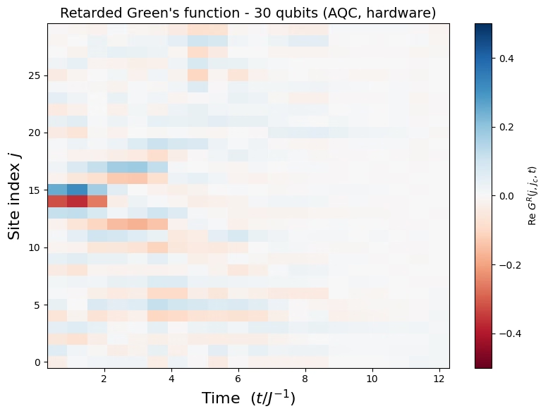
과학 코드를 변경하지 않고도 동일한 워크플로가 확장됩니다: 30사이트 사슬, 두 배의 Trotter 깊이(20단계), 나중의 더 얽힌 단계에 대해 더 깊은 앤사츠를 사용하는 압축 계획, 그리고 함수의 내장 오류 완화(동적 디커플링, Pauli 트월링, 트월링된 판독 오류 소거(TREX))를 사용한 IBM Quantum 프로세서에서의 실행입니다. 설정에서 가져온 fn 핸들을 재사용하여 시뮬레이터 예제와 동일한 네 단계를 살펴봅니다.
| 소규모 | 대규모 | |
|---|---|---|
| 큐비트 | 10 | 30 |
| Trotter 단계 | 10 | 20 |
| AQC 압축 단계 (1계층 + 2계층) | 3 + 2 = 5 | 6 + 4 = 10 |
| 바닥 상태 앤사츠 계층 | 3 | 5 |
| MPS 최대 결합 차원 | 32 | 128 |
| 백엔드 | statevector | DD, Pauli 트월링, TREX가 적용된 QPU |
1단계: 고전적 입력을 양자 문제로 매핑하기
동일한 KCuF 하이젠베르크 SparsePauliOp를 구축하고 바닥 상태를 준비하는데, 이번에는 더 긴 사슬을 위해 더 깊은 gs_layers=5 앤사츠를 사용한 다음 중앙 사이트에서 중성자 킥을 내장합니다. 이는 소규모 매핑과 동일하지만 에서 이루어집니다.
10사이트 실행보다 더 낮은 바닥 상태 충실도가 예상됩니다: 여기서는 약 0.82인 반면 더 작은 사슬에서는 0.98인데, 이는 다섯 개의 HVA 계층이 30사이트 바닥 상태를 완전히 포착할 수 없기 때문입니다. 이는 실패라기보다는 예상되는 것이며, 원본 튜토리얼도 동일한 이유로 50사이트에서 약 0.65를 받아들입니다. gs_layers 또는 COBYQA 반복 상한을 높이면 추가적인 고전적 비용으로 이를 개선할 수 있습니다.
n = 30
dt = 0.6
time_steps = 20
center = n // 2 - 1

# Same MPS settings as the original large-scale run: a larger bond for the
# longer, more-entangled chain (shared by GS prep and AQC compression).
mps_max_bond = 128
mps_cutoff = 1e-8

# Same KCuF3 Hamiltonian and ground-state prep, on a larger chain
H = SparsePauliOp.from_sparse_list(
    [(p, [i, i + 1], 0.25) for i in range(n - 1) for p in ("XX", "YY", "ZZ")],
    num_qubits=n,
)
gs_circuit = prepare_ground_state(
    n, gs_layers=5, max_bond=mps_max_bond, cutoff=mps_cutoff
)
gs_circuit.rz(np.pi / 2, center)  # neutron kick at the center site
print(
    f"Prepared {n}-qubit ground state with the neutron kick at site {center}."
)
DMRG ground-state energy: -13.111355
GS fidelity: 0.8201
Prepared 30-qubit ground state with the neutron kick at site 14.
2단계와 3단계: 함수 템플릿으로 압축 및 실행하기
시뮬레이터 예제와 동일한 단일 호출이지만, 이번에는 backend_name이 IBM Quantum 프로세서를 가리키므로 함수가 그곳에서 트랜스파일하고 실행합니다. 압축 계획은 앤사츠 깊이를 다양화합니다: 처음 여섯 개의 (엉킴이 적은) Trotter 단계는 얕은 단일 계층 앤사츠로 압축되고, 다음 네 단계는 더 깊은 이중 계층 앤사츠로 압축되며, 20단계 중 나머지 10단계는 일반 Trotter로 실행됩니다. aqc_options는 더 길고 더 얽힌 사슬을 위해 MPS 결합 차원을 max_bond=128로 올리며(원본과 일치), 100회로 제한된 동일한 L-BFGS-B 최적화기를 유지합니다. estimator_options는 내장된 오류 완화 기능을 활성화합니다: 동적 디커플링(XY4), 게이트 트월링, TREX 측정 완화. 함수의 기본값은 TREX 학습 예산(measure_noise_learning)을 제외한 이 모든 것에서 이미 원본 튜토리얼과 일치합니다. 호출자가 제공한 estimator_options는 함수의 기본값에 병합되는 대신 전부 대체하므로, 키를 생략하면 함수의 기본값이 아닌 IBM Quantum Compute 기본값으로 대체되기 때문에 전체 블록이 여전히 작성되어 있습니다.
# Steps 2 + 3: the function compresses (varied ansatz) and executes on hardware.
job = fn.run(
    t_steps=time_steps,
    aqc_segments=[
        {
            "n_steps": 6,
            "ansatz_steps": 1,
        },  # early steps -> shallow 1-layer ansatz
        {
            "n_steps": 4,
            "ansatz_steps": 2,
        },  # later steps -> deeper 2-layer ansatz
    ],
    aqc_options={
        "max_bond": mps_max_bond,  # 128 for the longer chain
        "cutoff": mps_cutoff,
        "optimizer_settings": {
            "method": "L-BFGS-B",
            "jac": True,
            "options": {"maxiter": 100},
        },
    },
    dt=dt,
    hamiltonian=H,
    initial_state=gs_circuit,
    backend_name="ibm_pittsburgh",
    # Mitigation settings from the original tutorial. Only the two
    # measure_noise_learning values differ from the function's defaults; the rest
    # restates them, because a caller-supplied estimator_options dict replaces the
    # function's defaults wholesale rather than merging into them.
    estimator_options={
        "environment": {"job_tags": ["TUT-SNS"]},
        "dynamical_decoupling": {"enable": True, "sequence_type": "XY4"},
        "twirling": {
            "enable_gates": True,
            "num_randomizations": 1000,
            "shots_per_randomization": 128,
        },
        "resilience": {
            "measure_mitigation": True,
            "measure_noise_learning": {
                "num_randomizations": 32,
                "shots_per_randomization": 100,
            },
        },
    },
)
print("job ID (save this to reconnect later):", job.job_id)
job ID (save this to reconnect later): 43ed8d07-6d7d-4f33-b70a-7f31b765b310
대규모 실행은 빠르지 않으며, 대부분의 시간은 QPU가 아닌 고전적 처리에 소요됩니다. AQC 압축은 QPU에 도달하기 전에 함수 내부에서 실행됩니다: 30사이트에서 max_bond=128을 사용했을 때 이번 실행에서는 거의 4시간이 걸렸으며, 이 튜토리얼 상단의 사용량 추정치에 명시된 약 18분의 QPU 시간과 대조됩니다. 큐 대기 시간은 이 두 가지 시간 모두에 더해집니다. 실행되는 동안 이 노트북이나 커널을 열어 둘 필요는 없습니다.
이전 셀에서 출력된 작업 ID를 복사하여 저장하세요. 다음 세 개의 셀을 사용하면 나중에 작업을 다시 시작할 수 있습니다:
-
다시 연결하기, 새로운 커널 세션에서만 필요합니다: 설정 셀을 다시 실행하여
serverless를 재생성한 다음 저장한 ID로부터job핸들을 재구축하세요. 제출한 세션에 아직 있는 경우 이 셀을 건너뛰세요. 핸들이 이미 활성화되어 있기 때문입니다. -
상태 확인하기:
DONE이 보고될 때까지 다시 실행하세요. -
결과 가져오기: 상태가
DONE이 된 후에만 실행하세요.
다음 재연결 셀에는 자리 표시자가 있습니다. 이를 자신의 job_id로 바꾸세요:
# Reconnect to a previously submitted job by its ID. Only needed in a NEW kernel
# session; if you are still in the session where you submitted, the `job` handle
# from the preceding cell is already live, so skip this cell. Replace the ID that follows with your own.
job = serverless.get_job_by_id("<your job ID>")
# Check where the job is. Re-run this until it reports DONE before fetching the
# result in the following cell: QUEUED -> INITIALIZING -> RUNNING: OPTIMIZING_FOR_HARDWARE ->
# RUNNING: WAITING_FOR_QPU -> RUNNING: EXECUTING_QPU -> RUNNING: POST_PROCESSING
# -> DONE.
print(job.status())
DONE
# Run this only once the preceding status cell reports DONE. result() blocks until
# the job finishes, so calling it earlier just waits (possibly for hours).
result = job.result()
print(
    "AQC fidelities:",
    {k: round(v, 4) for k, v in result["metadata"]["aqc_fidelities"].items()},
)

ev = np.array(result["expectation_values"])
Gjjc = ev[1:]  # drop the t = 0 row -> shape (time_steps, n)
AQC fidelities: {'1': 1.0, '2': 0.9994, '3': 0.9944, '4': 0.9853, '5': 0.9747, '6': 0.959, '7': 0.9495, '8': 0.9542, '9': 0.9533, '10': 0.9451}
4단계: 후처리하고 원하는 고전적 형식으로 결과 반환
시뮬레이터 실행과 동일한 후처리입니다: 그린 함수를 푸리에 변환하여 로 만들고, 거울 대칭화한 다음 음수 값을 잘라냅니다. 더 긴 사슬과 진화로 인해 이중 스피논 연속체가 훨씬 더 잘 해상됩니다. 점선 경계 사이의 밴드를 채워야 하며, 근처에서 가장 밝습니다.
n = result["metadata"]["n"]
q_res, w_res = 100, 100
spectrum = get_spectrum(n, Gjjc, dt, time_steps, q_res, w_res)
spectrum = -(spectrum + spectrum[:, ::-1]) / 2  # mirror symmetry
spectrum = np.clip(spectrum, a_min=0, a_max=None)  # clip negatives

plot_green(
    n,
    Gjjc,
    time_steps,
    dt,
    title=f"Retarded Green's function - {n} qubits (AQC, hardware)",
)
plot_spectrum(
    spectrum,
    dt,
    q_res,
    w_res,
    lower_bound=True,
    upper_bound=True,
    title=f"Dynamical structure factor - {n} qubits (AQC, hardware)",
)
부록
앞선 하드웨어 예제는 단일 사슬 길이를 실행합니다. 다음에 나오는 세 개의 스펙트럼은 다른 모든 입력을 고정한 채 ibm_pittsburgh에서 10, 20, 30사이트로 실행한 동일한 워크플로의 이전 하드웨어 실행에서 가져온 것입니다: dt = 0.6에서의 20단계 Trotter, 6개의 1계층과 4개의 2계층 AQC 압축 단계의 압축 계획, 그리고 max_bond = 128. 이것들은 앞선 셀의 출력이 아니라 기록된 결과입니다.
세 가지 크기 모두 동일한 설정이 사용되므로 스펙트럼을 직접 비교할 수 있습니다. 사슬 길이별로 조정하면(예: 더 많은 바닥 상태 앤사츠 계층이나 더 큰 max_bond) 여기 표시된 것보다 더 나은 결과를 얻을 수 있습니다.
다음 단계
-
이 워크플로를 자신의 시스템에 적용하세요: 이 함수는 임의의 1차원 최근접 이웃
SparsePauliOp를 받아들이므로, 다른 사슬 해밀토니안, 초기 상태, 또는 관측량 집합도 동일한 PRE → FUNCTION → POST 파이프라인으로 실행됩니다. 전체 입출력 계약은 GitHub의 AQC Dynamics Template에서 확인하세요. -
이 벤치마크의 출처가 되는 논문을 읽어보세요: Lee 외., Benchmarking quantum simulation with neutron-scattering experiments (arXiv:2603.15608).
-
이 워크플로가 배포된 함수 템플릿으로 이식한 인라인 워크플로인 원본 "중성자 산란 시뮬레이션하기" 튜토리얼과 비교해보세요.
-
하드웨어 실행에 적용된 오류 완화 및 억제 기법을 더 깊이 알아보세요: 동적 디커플링, Pauli 트월링, TREX.