양자 시뮬레이션

참고

Yukio Kawashima (2024년 5월 30일)

원본 강의의 PDF를 다운로드하세요. 일부 코드 스니펫은 정적 이미지이므로 더 이상 사용되지 않을 수 있습니다.

이 실험을 실행하는 데 소요되는 대략적인 QPU 시간은 7초입니다.

(이 노트북은 현재 더 이상 사용되지 않는 Qiskit Algorithms의 튜토리얼 노트북에서 주로 가져왔습니다.)

1. 소개

트로터화(Trotterization)는 실시간 시간 발전 기법으로, 특정 시간 슬라이스 동안 시스템의 시간 발전을 근사하도록 선택된 양자 Gate 또는 여러 Gate를 연속적으로 적용하는 방식입니다. 슈뢰딩거 방정식에 따르면, 초기 상태 $\vert\psi(0)\rangle$에서 시작하는 시스템의 시간 발전은 다음과 같은 형태를 취합니다:

$$\vert \psi(t) \rangle = e^{-i H t} \vert \psi(0) \rangle \text{,}$$

여기서 $H$는 시스템을 지배하는 시간 독립적인 해밀토니안입니다. $n$개의 Qubit에 작용하는 파울리 항의 텐서곱을 $P_j$라 할 때, 해밀토니안을 파울리 항들의 가중합으로 $H=\sum_j a_j P_j$와 같이 쓸 수 있다고 가정합니다. 이 파울리 항들은 서로 교환 가능(commute)할 수도 있고, 그렇지 않을 수도 있습니다. $t=0$일 때의 상태가 주어졌을 때, 양자 컴퓨터를 사용하여 이후 시각 $|\psi(t)\rangle$에서의 시스템 상태를 어떻게 구할 수 있을까요? 연산자의 지수 함수는 테일러 급수를 통해 가장 쉽게 이해할 수 있습니다:

$$e^{-i H t} = 1-iHt-\frac{1}{2}H^2t^2+...$$

$e^{iZ}$와 같이 매우 기본적인 지수 함수는 소수의 양자 Gate 집합을 사용하여 양자 컴퓨터에서 쉽게 구현할 수 있습니다. 하지만 관심 있는 대부분의 해밀토니안은 단일 항만으로 구성되지 않고, 여러 항을 포함합니다. $H = H_1+H_2$일 때 어떤 일이 일어나는지 살펴보겠습니다:

$$e^{-i H t} = 1-i(H_1+H_2)t-\frac{1}{2}(H_1+H_2)^2t^2+...$$

$H_1$과 $H_2$가 교환 가능한 경우, 숫자나 변수 $a$, $b$에서도 성립하는 친숙한 결과를 얻습니다:

$$e^{-i (a+b) t} = e^{-i a t}e^{-i b t}$$

그러나 연산자들이 교환 가능하지 않은 경우, 테일러 급수에서 항들을 이런 방식으로 단순화하기 위해 재배열할 수 없습니다. 따라서 복잡한 해밀토니안을 양자 Gate로 표현하는 것은 어려운 문제입니다.

한 가지 해결책은 테일러 전개에서 1차 항이 지배적이 될 만큼 매우 작은 시간 $t$를 고려하는 것입니다. 그 가정 하에서:

$$e^{-i (H_1+H_2) t} \approx 1-i(H_1+H_2)t \approx (1-i H_1 t)(1-i H_2 t) \approx e^{-i H_1 t}e^{-i H_2 t}$$

물론, 더 긴 시간 동안 상태를 발전시켜야 할 수도 있습니다. 이는 이러한 작은 시간 단계를 여러 번 반복함으로써 달성할 수 있습니다. 이 과정을 트로터화(Trotterization)라고 합니다:

$$\vert \psi(t) \rangle \approx \left(\prod_j e^{-i a_j P_j t/r} \right)^r \vert\psi(0) \rangle \text{,}$$

여기서 $t/r$은 우리가 선택하는 시간 슬라이스(발전 단계)입니다. 그 결과, $r$번 적용할 Gate가 생성됩니다. 시간 단계가 작을수록 더 정확한 근사를 얻을 수 있습니다. 그러나 이는 더 깊은 Circuit으로 이어지고, 실제로는 더 많은 오류가 누적됩니다(근미래 양자 장치에서 무시할 수 없는 문제입니다).

오늘은 $N=2$ 및 $N=6$ 사이트의 선형 격자에서 이징 모델의 시간 발전을 공부합니다. 이 격자는 가장 가까운 이웃하고만 상호작용하는 스핀 $\sigma_i$의 배열로 구성됩니다. 이 스핀은 두 가지 방향을 가질 수 있습니다: $\uparrow$와 $\downarrow$로, 각각 자화값 $+1$과 $-1$에 해당합니다.

$$H = - J \sum_{i=0}^{N-2} Z_i Z_{i+1} - h \sum_{i=0}^{N-1} X_i \text{,}$$

여기서 $J$는 상호작용 에너지를, $h$는 외부 자기장의 크기를 나타냅니다(위에서는 x 방향이지만, 이를 수정할 예정입니다). 이 식을 파울리 행렬로 작성하고 외부 자기장이 횡방향에 대해 각도 $\alpha$를 이루는 경우를 고려하면,

$$H = -J \sum_{i=0}^{N-2} Z_i Z_{i+1} -h \sum_{i=0}^{N-1} (\sin\alpha Z_i + \cos\alpha X_i) \text{.}$$

이 해밀토니안은 외부 자기장의 효과를 쉽게 연구할 수 있다는 점에서 유용합니다. 계산 기저에서 시스템은 다음과 같이 인코딩됩니다:

양자 상태	스핀 표현
$\lvert 0 0 0 0 \rangle$	$\uparrow\uparrow\uparrow\uparrow$
$\lvert 1 0 0 0 \rangle$	$\downarrow\uparrow\uparrow\uparrow$
$\ldots$	$\ldots$
$\lvert 1 1 1 1 \rangle$	$\downarrow\downarrow\downarrow\downarrow$

이제 이러한 양자 시스템의 시간 발전을 탐구해 보겠습니다. 구체적으로, 자화와 같은 시스템의 특정 속성들의 시간 발전을 시각화할 것입니다.

1.1 요구 사항

이 튜토리얼을 시작하기 전에 다음이 설치되어 있는지 확인하세요:

• Qiskit SDK v1.2 이상 ( pip install qiskit )
• Qiskit Runtime v0.30 이상 ( pip install qiskit-ibm-runtime )
• Numpy v1.24.1 이상 < 2 ( pip install numpy )

1.2 라이브러리 가져오기

유용할 수 있는 일부 라이브러리(MatrixExponential, QDrift)는 현재 노트북에서 사용되지 않지만 포함되어 있습니다. 시간이 있다면 직접 사용해 보세요!

# Added by doQumentation — required packages for this notebook
!pip install -q matplotlib numpy qiskit qiskit-ibm-runtime

# Check the version of Qiskit
import qiskit

qiskit.__version__

'2.0.2'

# Import the qiskit library
import numpy as np
import matplotlib.pylab as plt
import warnings

from qiskit import QuantumCircuit
from qiskit.circuit.library import PauliEvolutionGate
from qiskit.primitives import StatevectorEstimator
from qiskit.quantum_info import Statevector, SparsePauliOp
from qiskit.synthesis import (
    SuzukiTrotter,
    LieTrotter,
)
from qiskit.transpiler.preset_passmanagers import generate_preset_pass_manager

from qiskit_ibm_runtime import QiskitRuntimeService, SamplerV2

warnings.filterwarnings("ignore")

2. 문제 매핑하기

2.1 횡방향 자기장 이징 해밀토니안 정의하기

여기서는 1차원 횡방향 자기장 이징 모델을 다룹니다.

먼저, 시스템 파라미터 $N$, $J$, $h$, $\alpha$를 입력받아 해밀토니안을 SparsePauliOp으로 반환하는 함수를 만들겠습니다. SparsePauliOp은 가중치가 부여된 Pauli 항들로 연산자를 희소하게 표현한 것입니다.

def get_hamiltonian(nqubits, J, h, alpha):
    # List of Hamiltonian terms as 3-tuples containing
    # (1) the Pauli string,
    # (2) the qubit indices corresponding to the Pauli string,
    # (3) the coefficient.
    ZZ_tuples = [("ZZ", [i, i + 1], -J) for i in range(0, nqubits - 1)]
    Z_tuples = [("Z", [i], -h * np.sin(alpha)) for i in range(0, nqubits)]
    X_tuples = [("X", [i], -h * np.cos(alpha)) for i in range(0, nqubits)]

    # We create the Hamiltonian as a SparsePauliOp, via the method
    # `from_sparse_list`, and multiply by the interaction term.
    hamiltonian = SparsePauliOp.from_sparse_list(
        [*ZZ_tuples, *Z_tuples, *X_tuples], num_qubits=nqubits
    )
    return hamiltonian.simplify()

해밀토니안 정의하기

예시로, 크기 $N=6$, $J=0.2$, $h=1.2$, $\alpha=\frac{\pi}{8.0}$인 시스템을 고려합니다.

n_qubits = 6

hamiltonian = get_hamiltonian(nqubits=n_qubits, J=0.2, h=1.2, alpha=np.pi / 8.0)
hamiltonian

SparsePauliOp(['IIIIZZ', 'IIIZZI', 'IIZZII', 'IZZIII', 'ZZIIII', 'IIIIIZ', 'IIIIZI', 'IIIZII', 'IIZIII', 'IZIIII', 'ZIIIII', 'IIIIIX', 'IIIIXI', 'IIIXII', 'IIXIII', 'IXIIII', 'XIIIII'],
              coeffs=[-0.2       +0.j, -0.2       +0.j, -0.2       +0.j, -0.2       +0.j,
 -0.2       +0.j, -0.45922012+0.j, -0.45922012+0.j, -0.45922012+0.j,
 -0.45922012+0.j, -0.45922012+0.j, -0.45922012+0.j, -1.10865544+0.j,
 -1.10865544+0.j, -1.10865544+0.j, -1.10865544+0.j, -1.10865544+0.j,
 -1.10865544+0.j])

2.2 시간 진화 시뮬레이션 파라미터 설정하기

여기서는 세 가지 Trotterization 기법을 고려합니다.

• Lie–Trotter (1차)
• 2차 Suzuki–Trotter
• 4차 Suzuki–Trotter

뒤의 두 가지는 연습 문제와 부록에서 사용됩니다.

num_timesteps = 60
evolution_time = 30.0
dt = evolution_time / num_timesteps
product_formula_lt = LieTrotter()
product_formula_st2 = SuzukiTrotter(order=2)
product_formula_st4 = SuzukiTrotter(order=4)

2.3 양자 Circuit 준비 1 (초기 상태)

초기 상태를 생성합니다. 여기서는 스핀 배열 $\uparrow\uparrow\downarrow\downarrow\uparrow\uparrow$으로 시작합니다.

initial_circuit = QuantumCircuit(n_qubits)
initial_circuit.prepare_state("001100")
# Change reps and see the difference when you decompose the circuit
initial_circuit.decompose(reps=1).draw("mpl")

2.4 양자 Circuit 준비 2 (단일 시간 진화 Circuit)

여기서는 Lie–Trotter를 사용하여 단일 시간 스텝에 대한 Circuit을 구성합니다.

Lie 곱 공식(1차)은 LieTrotter 클래스에 구현되어 있습니다. 1차 공식은 서론에서 언급한 근사, 즉 합의 행렬 지수를 행렬 지수들의 곱으로 근사하는 것으로 구성됩니다.

$$e^{H_1+H_2} \approx e^{H_1} e^{H_2}$$

앞서 언급했듯이, Circuit이 매우 깊어지면 오류가 누적되어 현대 양자 컴퓨터에서 문제를 일으킵니다. 2-Qubit Gate는 단일 Qubit Gate보다 오류율이 높기 때문에, 특히 중요한 지표는 2-Qubit Circuit 깊이입니다. 실질적으로 중요한 것은 트랜스파일 후의 2-Qubit Circuit 깊이입니다(그 Circuit이 실제로 양자 컴퓨터에서 실행되는 것이기 때문입니다). 하지만 지금은 시뮬레이터를 사용하더라도, 이 Circuit의 연산 수를 세는 습관을 들이도록 합시다.

single_step_evolution_gates_lt = PauliEvolutionGate(
    hamiltonian, dt, synthesis=product_formula_lt
)
single_step_evolution_lt = QuantumCircuit(n_qubits)
single_step_evolution_lt.append(
    single_step_evolution_gates_lt, single_step_evolution_lt.qubits
)

print(
    f"""
Trotter step with Lie-Trotter
-----------------------------
Depth: {single_step_evolution_lt.decompose(reps=3).depth()}
Gate count: {len(single_step_evolution_lt.decompose(reps=3))}
Nonlocal gate count: {single_step_evolution_lt.decompose(reps=3).num_nonlocal_gates()}
Gate breakdown: {", ".join([f"{k.upper()}: {v}" for k, v in single_step_evolution_lt.decompose(reps=3).count_ops().items()])}
"""
)
single_step_evolution_lt.decompose(reps=3).draw("mpl", fold=-1)

Trotter step with Lie-Trotter
-----------------------------
Depth: 17
Gate count: 27
Nonlocal gate count: 10
Gate breakdown: U3: 12, CX: 10, U1: 5

2.5 측정할 연산자 설정하기

자기화 연산자 $\sum_i \langle Z_i \rangle / N$와 평균 스핀 상관 연산자 $\sum_i \langle Z_i Z_{i+1} \rangle/ (N - 1)$를 정의합니다.

magnetization = (
    SparsePauliOp.from_sparse_list(
        [("Z", [i], 1.0) for i in range(0, n_qubits)], num_qubits=n_qubits
    )
    / n_qubits
)
correlation = SparsePauliOp.from_sparse_list(
    [("ZZ", [i, i + 1], 1.0) for i in range(0, n_qubits - 1)], num_qubits=n_qubits
) / (n_qubits - 1)
print("magnetization : ", magnetization)
print("correlation : ", correlation)

magnetization :  SparsePauliOp(['IIIIIZ', 'IIIIZI', 'IIIZII', 'IIZIII', 'IZIIII', 'ZIIIII'],
              coeffs=[0.16666667+0.j, 0.16666667+0.j, 0.16666667+0.j, 0.16666667+0.j,
 0.16666667+0.j, 0.16666667+0.j])
correlation :  SparsePauliOp(['IIIIZZ', 'IIIZZI', 'IIZZII', 'IZZIII', 'ZZIIII'],
              coeffs=[0.2+0.j, 0.2+0.j, 0.2+0.j, 0.2+0.j, 0.2+0.j])

2.6 시간 진화 시뮬레이션 수행하기

에너지(해밀토니안의 기댓값), 자기화(자기화 연산자의 기댓값), 평균 스핀 상관(평균 스핀 상관 연산자의 기댓값)을 모니터링합니다. Qiskit의 StatevectorEstimator(EstimatorV2) 프리미티브는 관측량의 기댓값 $\langle\psi\vert\hat{O}\vert\psi\rangle$을 추정합니다.

# Initiate the circuit
evolved_state = QuantumCircuit(initial_circuit.num_qubits)
# Start from the initial spin configuration
evolved_state.append(initial_circuit, evolved_state.qubits)
# Initiate Estimator (V2)
estimator = StatevectorEstimator()
# Set number of shots
shots = 10000
# Translate the precision required from the number of shots
precision = np.sqrt(1 / shots)
energy_list = []
mag_list = []
corr_list = []
# Estimate expectation values for t=0.0
job = estimator.run(
    [(evolved_state, [hamiltonian, magnetization, correlation])], precision=precision
)
# Get estimated expectation values
evs = job.result()[0].data.evs
energy_list.append(evs[0])
mag_list.append(evs[1])
corr_list.append(evs[2])
# Start time evolution
for n in range(num_timesteps):
    # Expand the circuit to describe delta-t
    evolved_state.append(single_step_evolution_gates_lt, evolved_state.qubits)
    # Estimate expectation values at delta-t
    job = estimator.run(
        [(evolved_state, [hamiltonian, magnetization, correlation])],
        precision=precision,
    )
    # Retrieve results (expectation values)
    evs = job.result()[0].data.evs
    energy_list.append(evs[0])
    mag_list.append(evs[1])
    corr_list.append(evs[2])
# Transform the list of expectation values (at each time step) to arrays
energy_array = np.array(energy_list)
mag_array = np.array(mag_list)
corr_array = np.array(corr_list)

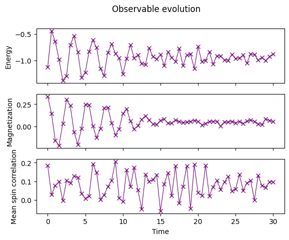
2.7 관측량의 시간 진화 플롯하기

측정한 기댓값을 시간에 대해 플롯합니다.

fig, axes = plt.subplots(3, sharex=True)
times = np.linspace(0, evolution_time, num_timesteps + 1)  # includes initial state
axes[0].plot(
    times,
    energy_array,
    label="First order",
    marker="x",
    c="darkmagenta",
    ls="-",
    lw=0.8,
)
axes[1].plot(
    times, mag_array, label="First order", marker="x", c="darkmagenta", ls="-", lw=0.8
)
axes[2].plot(
    times, corr_array, label="First order", marker="x", c="darkmagenta", ls="-", lw=0.8
)
axes[0].set_ylabel("Energy")
axes[1].set_ylabel("Magnetization")
axes[2].set_ylabel("Mean spin correlation")
axes[2].set_xlabel("Time")
fig.suptitle("Observable evolution")

Text(0.5, 0.98, 'Observable evolution')

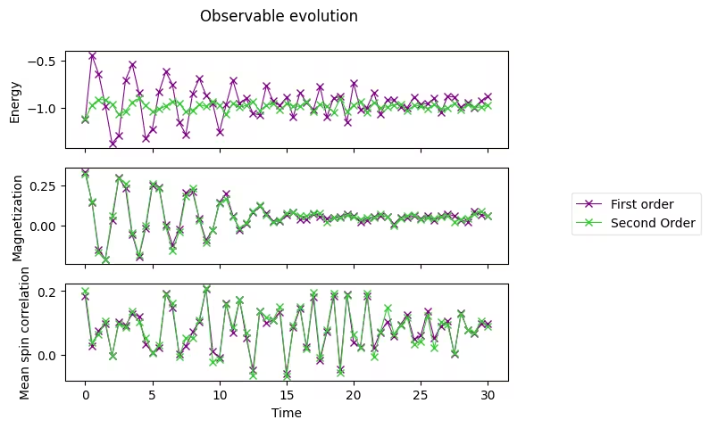
3. 연습 1. 2차 Suzuki–Trotter를 사용한 시뮬레이션 수행

위에서 보여준 Lie–Trotter 예시를 참고하여, 2차 Suzuki–Trotter로 시뮬레이션을 수행해 보겠습니다.

Qiskit에서 2차 Suzuki-Trotter는 SuzukiTrotter 클래스를 통해 사용할 수 있습니다. 이 공식을 사용하면 2차 분해는 다음과 같습니다.

$$e^{H_1+H_2} \approx e^{H_1/2}e^{H_2}e^{H_1/2}$$

3.1 단일 시간 스텝을 위한 Circuit 구성

product_formula_st2 (SuzukiTrotter(order=2))를 사용하여 2차 Suzuki–Trotter 기반의 단일 시간 스텝 Circuit을 구성합니다. 또한 게이트 수와 Circuit 깊이를 계산하여 Lie–Trotter와 비교해 보세요.

# Modify the line below (Use PauliEvolutionGate)
single_step_evolution_gates_st2 = PauliEvolutionGate(
    hamiltonian, dt, synthesis=product_formula_st2
)
single_step_evolution_st2 = QuantumCircuit(n_qubits)
single_step_evolution_st2.append(
    single_step_evolution_gates_st2, single_step_evolution_st2.qubits
)
# Let us print some stats
print(
    f"""
Trotter step with second-order Suzuki-Trotter
-----------------------------
Depth: {single_step_evolution_st2.decompose(reps=3).depth()}
Gate count: {len(single_step_evolution_st2.decompose(reps=3))}
Nonlocal gate count: {single_step_evolution_st2.decompose(reps=3).num_nonlocal_gates()}
Gate breakdown: {", ".join([f"{k.upper()}: {v}" for k, v in single_step_evolution_st2.decompose(reps=3).count_ops().items()])}
"""
)
single_step_evolution_st2.decompose(reps=2).draw("mpl", fold=-1)

Trotter step with second-order Suzuki-Trotter
-----------------------------
Depth: 34
Gate count: 53
Nonlocal gate count: 20
Gate breakdown: U3: 23, CX: 20, U1: 10

3.2 시간 진화 시뮬레이션 수행

2차 Suzuki–Trotter를 사용하여 시간 진화를 수행합니다.

# Initiate the circuit
evolved_state = QuantumCircuit(initial_circuit.num_qubits)
# Start from the initial spin configuration
evolved_state.append(initial_circuit, evolved_state.qubits)
# Initiate Estimator (V2)
estimator = StatevectorEstimator()
# Set number of shots
shots = 10000
# Translate the precision required from the number of shots
precision = np.sqrt(1 / shots)
energy_list_st2 = []
mag_list_st2 = []
corr_list_st2 = []
# Estimate expectation values for t=0.0
job = estimator.run(
    [(evolved_state, [hamiltonian, magnetization, correlation])], precision=precision
)
# Get estimated expectation values
evs = job.result()[0].data.evs
energy_list_st2.append(evs[0])
mag_list_st2.append(evs[1])
corr_list_st2.append(evs[2])
# Start time evolution
for n in range(num_timesteps):
    # Expand the circuit to describe delta-t
    evolved_state.append(single_step_evolution_gates_st2, evolved_state.qubits)
    # Estimate expectation values at delta-t
    job = estimator.run(
        [(evolved_state, [hamiltonian, magnetization, correlation])],
        precision=precision,
    )
    # Retrieve results (expectation values)
    evs = job.result()[0].data.evs
    energy_list_st2.append(evs[0])
    mag_list_st2.append(evs[1])
    corr_list_st2.append(evs[2])
# Transform the list of expectation values (at each time step) to arrays
energy_array_st2 = np.array(energy_list_st2)
mag_array_st2 = np.array(mag_list_st2)
corr_array_st2 = np.array(corr_list_st2)

3.3 2차 Suzuki–Trotter 결과 플롯

axes[0].plot(
    times,
    energy_array_st2,
    label="Second Order",
    marker="x",
    c="limegreen",
    ls="-",
    lw=0.8,
)
axes[1].plot(
    times,
    mag_array_st2,
    label="Second Order",
    marker="x",
    c="limegreen",
    ls="-",
    lw=0.8,
)
axes[2].plot(
    times,
    corr_array_st2,
    label="Second Order",
    marker="x",
    c="limegreen",
    ls="-",
    lw=0.8,
)

# Replace the legend
# legend.remove()
legend = fig.legend(
    *axes[0].get_legend_handles_labels(),
    bbox_to_anchor=(1.0, 0.5),
    loc="center left",
    framealpha=0.5,
)
fig

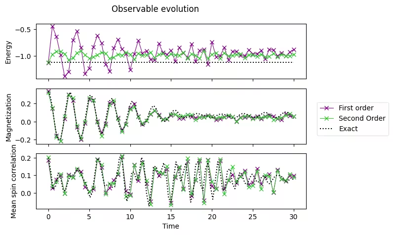
3.4 정확한 결과와 비교

아래 데이터는 클래식 컴퓨터에서 미리 계산한 정확한 결과입니다.

exact_times = np.array(
    [
        0.0,
        0.3,
        0.6,
        0.8999999999999999,
        1.2,
        1.5,
        1.7999999999999998,
        2.1,
        2.4,
        2.6999999999999997,
        3.0,
        3.3,
        3.5999999999999996,
        3.9,
        4.2,
        4.5,
        4.8,
        5.1,
        5.3999999999999995,
        5.7,
        6.0,
        6.3,
        6.6,
        6.8999999999999995,
        7.199999999999999,
        7.5,
        7.8,
        8.1,
        8.4,
        8.7,
        9.0,
        9.299999999999999,
        9.6,
        9.9,
        10.2,
        10.5,
        10.799999999999999,
        11.1,
        11.4,
        11.7,
        12.0,
        12.299999999999999,
        12.6,
        12.9,
        13.2,
        13.5,
        13.799999999999999,
        14.1,
        14.399999999999999,
        14.7,
        15.0,
        15.299999999999999,
        15.6,
        15.899999999999999,
        16.2,
        16.5,
        16.8,
        17.099999999999998,
        17.4,
        17.7,
        18.0,
        18.3,
        18.599999999999998,
        18.9,
        19.2,
        19.5,
        19.8,
        20.099999999999998,
        20.4,
        20.7,
        21.0,
        21.3,
        21.599999999999998,
        21.9,
        22.2,
        22.5,
        22.8,
        23.099999999999998,
        23.4,
        23.7,
        24.0,
        24.3,
        24.599999999999998,
        24.9,
        25.2,
        25.5,
        25.8,
        26.099999999999998,
        26.4,
        26.7,
        27.0,
        27.3,
        27.599999999999998,
        27.9,
        28.2,
        28.5,
        28.799999999999997,
        29.099999999999998,
        29.4,
        29.7,
        30.0,
    ]
)
exact_energy = np.array(
    [
        -1.1184402376762155,
        -1.1184402376762157,
        -1.1184402376762157,
        -1.1184402376762148,
        -1.1184402376762153,
        -1.1184402376762155,
        -1.1184402376762148,
        -1.118440237676216,
        -1.118440237676216,
        -1.1184402376762166,
        -1.1184402376762148,
        -1.118440237676216,
        -1.1184402376762153,
        -1.1184402376762148,
        -1.118440237676217,
        -1.118440237676215,
        -1.1184402376762161,
        -1.1184402376762157,
        -1.118440237676217,
        -1.1184402376762161,
        -1.1184402376762137,
        -1.1184402376762161,
        -1.1184402376762161,
        -1.118440237676218,
        -1.1184402376762155,
        -1.1184402376762166,
        -1.1184402376762155,
        -1.1184402376762137,
        -1.1184402376762186,
        -1.1184402376762215,
        -1.1184402376762148,
        -1.118440237676216,
        -1.1184402376762166,
        -1.1184402376762148,
        -1.1184402376762121,
        -1.1184402376762166,
        -1.1184402376762181,
        -1.1184402376762137,
        -1.1184402376762148,
        -1.1184402376762193,
        -1.1184402376762108,
        -1.1184402376762144,
        -1.118440237676217,
        -1.1184402376762197,
        -1.1184402376762153,
        -1.1184402376762161,
        -1.1184402376762184,
        -1.1184402376762126,
        -1.118440237676214,
        -1.118440237676214,
        -1.1184402376762161,
        -1.118440237676212,
        -1.1184402376762164,
        -1.118440237676217,
        -1.1184402376762121,
        -1.1184402376762157,
        -1.1184402376762212,
        -1.1184402376762217,
        -1.1184402376762206,
        -1.118440237676222,
        -1.1184402376762166,
        -1.118440237676212,
        -1.1184402376762137,
        -1.11844023767622,
        -1.1184402376762206,
        -1.118440237676219,
        -1.1184402376762153,
        -1.1184402376762164,
        -1.118440237676209,
        -1.1184402376762144,
        -1.1184402376762161,
        -1.118440237676216,
        -1.1184402376762173,
        -1.118440237676214,
        -1.1184402376762093,
        -1.1184402376762184,
        -1.1184402376762126,
        -1.118440237676213,
        -1.1184402376762195,
        -1.1184402376762095,
        -1.1184402376762075,
        -1.1184402376762197,
        -1.1184402376762141,
        -1.1184402376762146,
        -1.1184402376762184,
        -1.118440237676218,
        -1.1184402376762224,
        -1.118440237676219,
        -1.118440237676218,
        -1.1184402376762206,
        -1.1184402376762168,
        -1.118440237676221,
        -1.118440237676218,
        -1.1184402376762148,
        -1.1184402376762106,
        -1.1184402376762173,
        -1.118440237676216,
        -1.118440237676216,
        -1.1184402376762113,
        -1.1184402376762275,
        -1.1184402376762195,
    ]
)
exact_magnetization = np.array(
    [
        0.3333333333333333,
        0.26316769633415005,
        0.0912947227110664,
        -0.09317712543141576,
        -0.20391854332115245,
        -0.19318196655046493,
        -0.06411527074401464,
        0.12558269854206197,
        0.28252754464640606,
        0.3264196194042506,
        0.2361586169847769,
        0.060894367906122224,
        -0.10842387093076275,
        -0.18636359582538073,
        -0.1338364343947887,
        0.020284606520827753,
        0.19151142743926025,
        0.2905341647678381,
        0.2723014646745304,
        0.15147481733047252,
        -0.008179102877790292,
        -0.1242999208732406,
        -0.1372529247781061,
        -0.04083616185958952,
        0.11066094926716476,
        0.23140661570567636,
        0.2587109403786205,
        0.1868237670027325,
        0.061201779383143744,
        -0.051391248969654205,
        -0.09843899603365061,
        -0.061297056158849166,
        0.04199010081939773,
        0.15861461430963147,
        0.22336830674799552,
        0.20179555623336537,
        0.11407111438609417,
        0.01609419104778282,
        -0.04239611796730001,
        -0.04249123521065924,
        0.008850291714888112,
        0.08780898151558082,
        0.1561486776507056,
        0.17627348772811832,
        0.13870676179652253,
        0.07205869195282538,
        0.018300003064909465,
        0.0001095640839572417,
        0.015157929316037586,
        0.05077755280969454,
        0.09245534457650838,
        0.12206907551110702,
        0.12284950557969157,
        0.09570215398601932,
        0.06294378255078983,
        0.045503313813986014,
        0.043389819499542556,
        0.046725117769796744,
        0.054956411358382404,
        0.0713814528253614,
        0.08743689703248492,
        0.08951216359166674,
        0.07878386475305985,
        0.06955669116405788,
        0.06639892435963689,
        0.05890378761746903,
        0.04541796525844558,
        0.0414221088331947,
        0.05499634106912299,
        0.07409418836014572,
        0.08371859070160165,
        0.08211623987959302,
        0.07615055161378328,
        0.06702584458783024,
        0.051891407742740085,
        0.038049378383635625,
        0.03825614149768043,
        0.054183218463525695,
        0.0753534475741016,
        0.08853147112587295,
        0.08767917178542013,
        0.07709383184439536,
        0.06308595032042386,
        0.0498812359204284,
        0.04299040064096167,
        0.04769159891460652,
        0.06483569572288776,
        0.08698035745435016,
        0.10047391641776235,
        0.09747255683203637,
        0.08098863187287358,
        0.05959496723987331,
        0.04383882265040485,
        0.04232138798062125,
        0.05720514169944535,
        0.08201306299870219,
        0.10274898262000469,
        0.10707552455080133,
        0.09210856128265357,
        0.06379922105742579,
        0.03624325103307953,
    ]
)
exact_correlation = np.array(
    [
        0.2,
        0.1247704225763532,
        0.01943938494098705,
        0.03854917181332821,
        0.11196616231067426,
        0.0906546700356683,
        0.01629373561896267,
        0.011352652889791095,
        0.0636185676540077,
        0.09543834437789013,
        0.10058518161011307,
        0.11829217731417431,
        0.1397812224038133,
        0.12316460402216707,
        0.08541383059335775,
        0.06144846844403662,
        0.020246372880505827,
        -0.02693683090021662,
        0.003919250903281282,
        0.1117419430168554,
        0.19676155181256794,
        0.18594408880783336,
        0.1002673802566004,
        0.03821525827438024,
        0.04485205090247377,
        0.05348102743040269,
        0.03160026140008638,
        0.033437649060464834,
        0.10486939975320728,
        0.20249469538955758,
        0.19735507621013149,
        0.0553097261765083,
        -0.04889114490131667,
        0.011685690974970964,
        0.11705971535823065,
        0.11681165998194759,
        0.06637091239560744,
        0.10936684225958895,
        0.20225454101061405,
        0.16284420833341812,
        -0.0025823294931362067,
        -0.0763416631752919,
        0.02985268630418397,
        0.15234468006771007,
        0.14606385406970995,
        0.0935341856492092,
        0.12325421854361143,
        0.17130422930386324,
        0.10383730044042278,
        -0.031333159406547614,
        -0.05241572078596815,
        0.07722509925347705,
        0.17642188574256007,
        0.12765340239966838,
        0.06309968945093776,
        0.11574687130499339,
        0.16978282647206913,
        0.0736143632571229,
        -0.05356602733119409,
        -0.0009649396796768892,
        0.15921620111869142,
        0.17760366431811037,
        0.04736297330213485,
        0.012122870263181897,
        0.13268065586830521,
        0.1728473023503636,
        0.03999259331072221,
        -0.036997053070222885,
        0.06951528580242439,
        0.1769169993516561,
        0.12290448295710298,
        0.012897784654866427,
        0.02859435620982225,
        0.12895847695150875,
        0.13629536955485938,
        0.05394621059822597,
        0.02298040588184324,
        0.07036499900317271,
        0.11706448623132719,
        0.10435285842074606,
        0.055721236329964965,
        0.04676334743672697,
        0.08417924910022263,
        0.10611161955304965,
        0.089304171047322,
        0.06098589533081194,
        0.06314519797488709,
        0.09431492621892917,
        0.09667836915967139,
        0.0651298357290882,
        0.05176966009147416,
        0.06727229484222669,
        0.08871788283607947,
        0.09907054249093444,
        0.09785167773502176,
        0.09277216140054353,
        0.07520999642062785,
        0.05894392248382922,
        0.07236135251622376,
        0.08608284185200156,
        0.07282922961856123,
    ]
)

axes[0].plot(exact_times, exact_energy, c="k", ls=":", label="Exact")
axes[1].plot(exact_times, exact_magnetization, c="k", ls=":", label="Exact")
axes[2].plot(exact_times, exact_correlation, c="k", ls=":", label="Exact")
# Replace the legend
legend.remove()
# Select the labels of only the first axis
legend = fig.legend(
    *axes[0].get_legend_handles_labels(),
    bbox_to_anchor=(1.0, 0.5),
    loc="center left",
    framealpha=0.5,
)
fig.tight_layout()
fig

4. 양자 하드웨어에서 실행하기

다음으로 양자 하드웨어에서 시간 진화 시뮬레이션을 실행해 봅니다. 격자 크기 N=2의 더 작은 문제를 다루고, $\alpha$ 매개변수를 변화시키면서 파동 함수 동역학의 차이를 살펴보겠습니다.

4.1 1단계. 고전적 입력을 양자 문제로 매핑하기

시뮬레이션의 초기 설정을 선택합니다:

n_qubits_2 = 2
dt_2 = 1.6
product_formula = LieTrotter(reps=1)

그런 다음 초기 Circuit을 설정합니다:

초기 스핀 배열은 "아래-위"로 설정합니다.

# We prepare an initial state ↓↑ (10).
# Note that Statevector and SparsePauliOp interpret the qubits from right to left
initial_circuit_2 = QuantumCircuit(n_qubits_2)
initial_circuit_2.prepare_state("10")
# Change reps and see the difference when you decompose the circuit
initial_circuit_2.decompose(reps=1).draw("mpl")

이제 이상적인 상태 벡터 시뮬레이터를 사용해 참조값을 계산합니다.

bar_width = 0.1
# initial_state = Statevector.from_label("10")
final_time = 1.6
eps = 1e-5

# We create the list of angles in radians, with a small epsilon
# the exactly longitudinal field, which would present no dynamics at all
alphas = np.linspace(-np.pi / 2 + eps, np.pi / 2 - eps, 5)

for i, alpha in enumerate(alphas):
    evolved_state_2 = QuantumCircuit(initial_circuit_2.num_qubits)
    evolved_state_2.append(initial_circuit_2, evolved_state_2.qubits)
    hamiltonian_2 = get_hamiltonian(nqubits=2, J=0.2, h=1.0, alpha=alpha)
    single_step_evolution_gates_2 = PauliEvolutionGate(
        hamiltonian_2, dt_2, synthesis=product_formula
    )
    evolved_state_2.append(single_step_evolution_gates_2, evolved_state_2.qubits)
    evolved_state_2 = Statevector(evolved_state_2)
    # Dictionary of probabilities
    amplitudes_dict = evolved_state_2.probabilities_dict()
    labels = list(amplitudes_dict.keys())
    values = list(amplitudes_dict.values())
    # Convert angle to degrees
    alpha_str = f"$\\alpha={int(np.round(alpha * 180 / np.pi))}^\\circ$"
    plt.bar(np.arange(4) + i * bar_width, values, bar_width, label=alpha_str, alpha=0.7)

plt.xticks(np.arange(4) + 2 * bar_width, labels)
plt.xlabel("Measurement")
plt.ylabel("Probability")
plt.suptitle(
    f"Measurement probabilities at $t={final_time}$, for various field angles $\\alpha$\n"
    f"Initial state: 10, Linear lattice of size $L=2$"
)
plt.legend()

<matplotlib.legend.Legend at 0x11c816590>

스핀이 $\downarrow\uparrow$인 배열로 초기화된 시스템, 즉 $\vert\psi(0)\rangle = \vert10\rangle$을 준비했습니다. 횡방향 필드($\alpha=0^\circ$) 아래에서 $t=1.6$만큼 진화시키면, 거의 확실하게 $\uparrow\downarrow$가 측정됩니다. 즉 스핀이 서로 뒤바뀝니다. (레이블은 오른쪽에서 왼쪽 순서로 해석됩니다.) 필드가 종방향($\alpha=\pm90^\circ$)이면 진화가 전혀 없으므로, 처음에 준비된 상태인 $\downarrow\uparrow$가 측정됩니다. 중간 각도인 $\alpha=\pm45^\circ$에서는 모든 조합이 서로 다른 확률로 측정되는데, 스핀 교환이 67%의 확률로 가장 높게 나타납니다.

하드웨어 실험용 Circuit 구성

circuit_list = []
for i, alpha in enumerate(alphas):
    evolved_state_2 = QuantumCircuit(initial_circuit_2.num_qubits)
    evolved_state_2.append(initial_circuit_2, evolved_state_2.qubits)
    hamiltonian_2 = get_hamiltonian(nqubits=2, J=0.2, h=1.0, alpha=alpha)
    single_step_evolution_gates_2 = PauliEvolutionGate(
        hamiltonian_2, dt_2, synthesis=product_formula
    )
    evolved_state_2.append(single_step_evolution_gates_2, evolved_state_2.qubits)
    evolved_state_2.measure_all()
    circuit_list.append(evolved_state_2)

4.2 2단계. 대상 하드웨어에 맞게 최적화하기

Backend를 지정합니다.

service = QiskitRuntimeService()
backend = service.least_busy(operational=True, simulator=False)
backend.name

'ibm_strasbourg'

그런 다음 선택한 Backend에 맞게 Circuit을 트랜스파일합니다.

pm = generate_preset_pass_manager(backend=backend, optimization_level=3)
circuit_isa = pm.run(circuit_list)

Circuit을 확인합니다.

circuit_isa[1].draw("mpl", idle_wires=False)

4.3 3단계. Qiskit Runtime 프리미티브로 실행하기

Qiskit의 Sampler(V2) 프리미티브는 측정된 비트 문자열의 횟수를 제공합니다.

sampler = SamplerV2(mode=backend)
job = sampler.run(circuit_isa)
job_id = job.job_id()
print("job id:", job_id)

job id: d13pswfmya70008ek070

결과를 저장합니다.

results = job.result()

4.4 4단계. 결과 후처리하기

비트 문자열의 히스토그램을 구성하여 파동 함수를 분석하고, 위에서 보여준 이상적인 값과 비교합니다.

list_temp = ["00", "01", "10", "11"]

for i, alpha in enumerate(alphas):
    # Dictionary of probabilities
    amplitudes_dict = results[i].data.meas.get_counts()
    values = []
    for str_temp in list_temp:
        values.append(
            amplitudes_dict[str_temp] / 4096.0
        )  # divided by default number of shots
    # Convert angle to degrees
    alpha_str = f"$\\alpha={int(np.round(alpha * 180 / np.pi))}^\\circ$"
    plt.bar(np.arange(4) + i * bar_width, values, bar_width, label=alpha_str, alpha=0.7)

plt.xticks(np.arange(4) + 2 * bar_width, labels)
plt.xlabel("Measurement")
plt.ylabel("Probabilities")
plt.suptitle(
    f"Measurement probabilities at $t={final_time}$, for various field angles $\\alpha$\n"
    f"Initial state: 10, Linear lattice of size $L=2$"
)
plt.legend()

<matplotlib.legend.Legend at 0x11d7af990>

여기서는 고차(4차) Suzuki–Trotter를 사용해 Circuit을 구성하는 예시를 보여줍니다. 위의 예시를 따라 4차 Suzuki–Trotter로 Circuit 시뮬레이션을 구성해 보세요.

4차 Suzuki–Trotter는 Qiskit의 SuzukiTrotter 클래스를 사용하면 됩니다. 4차는 다음 점화 관계를 이용해 계산할 수 있습니다. 아래 식에서 Suzuki–Trotter의 차수는 "2k"로 표기합니다.

$$\hat{U}_{ST(2k)}\left(t\right) = \left[ \hat{U}_{ST(2k-2)}\left(p_k t\right) \right]^2 \hat{U}_{ST(2k-2)}\left( (1- 4 p_k) t\right)\left[ \hat{U}_{ST(2k-2)}\left(p_k t\right) \right]^2$$ $$p_k = 1 / \left(4-4^{\frac{1}{2k-1}}\right)$$

단일 시간 스텝에 대한 Circuit 구성

product_formula_st4 (SuzukiTrotter(order=4))를 사용해 4차 Suzuki–Trotter로 단일 시간 스텝에 대한 Circuit을 구성하세요. 또한 Gate 수와 Circuit 깊이를 세어 Lie–Trotter 및 2차 Suzuki–Trotter와 비교해 보세요.

# Modify the line below (Use PauliEvolutionGate)
single_step_evolution_gates_st4 = PauliEvolutionGate(
    hamiltonian, dt, synthesis=product_formula_st4
)
single_step_evolution_st4 = QuantumCircuit(n_qubits)
single_step_evolution_st4.append(
    single_step_evolution_gates_st4, single_step_evolution_st4.qubits
)
# Let us print some stats
print(
    f"""
Trotter step with second-order Suzuki-Trotter
-----------------------------
Depth: {single_step_evolution_st4.decompose(reps=3).depth()}
Gate count: {len(single_step_evolution_st4.decompose(reps=3))}
Nonlocal gate count: {single_step_evolution_st4.decompose(reps=3).num_nonlocal_gates()}
Gate breakdown: {", ".join([f"{k.upper()}: {v}" for k, v in single_step_evolution_st4.decompose(reps=3).count_ops().items()])}
"""
)
single_step_evolution_st4.decompose(reps=2).draw("mpl", fold=-1)

Trotter step with second-order Suzuki-Trotter
-----------------------------
Depth: 170
Gate count: 265
Nonlocal gate count: 100
Gate breakdown: U3: 115, CX: 100, U1: 50

# Check Qiskit version
import qiskit

qiskit.__version__

'2.0.2'