양자 비트, 게이트, 그리고 회로

참고

Kifumi Numata (19 Apr 2024)

원본 강의 PDF를 다운로드하려면 여기를 클릭하세요. 정적 이미지로 구성된 일부 코드 스니펫은 더 이상 사용되지 않을 수 있습니다.

이 실험을 실행하는 데 걸리는 QPU 시간은 약 5초입니다.

1. 소개

비트, 게이트, 회로는 양자 컴퓨팅의 기본 구성 요소입니다. 여기서는 양자 비트와 게이트를 활용한 회로 모델로 양자 계산을 배우고, 중첩, 측정, 얽힘에 대해서도 복습합니다.

이번 강의에서 배울 내용:

• 단일 Qubit 게이트
• 블로흐 구
• 중첩
• 측정
• 2-Qubit 게이트와 얽힘 상태

강의 마지막에는 유틸리티 규모의 양자 컴퓨팅에서 필수적인 Circuit 깊이에 대해서도 배웁니다.

2. 다이어그램으로 나타내는 계산

Qubit 또는 비트를 사용할 때는, 입력을 원하는 출력으로 변환하기 위해 이들을 조작해야 합니다. 비트가 매우 적은 간단한 프로그램에서는 이 과정을 회로 다이어그램이라고 불리는 도식으로 나타내는 것이 유용합니다.

아래 왼쪽 그림은 고전 회로의 예시이고, 오른쪽 그림은 양자 Circuit의 예시입니다. 두 경우 모두 입력은 왼쪽에, 출력은 오른쪽에 있으며 연산은 기호로 표현됩니다. 연산에 사용되는 기호는 주로 역사적인 이유로 "게이트"라고 불립니다.

3. 단일 Qubit 양자 게이트

3.1 양자 상태와 블로흐 구

Qubit의 상태는 $|0\rangle$과 $|1\rangle$의 중첩으로 표현됩니다. 임의의 양자 상태는 다음과 같이 나타낼 수 있습니다.

$$|\psi\rangle =\alpha|0\rangle+ \beta|1\rangle$$

여기서 $\alpha$와 $\beta$는 $|\alpha|^2+|\beta|^2=1$을 만족하는 복소수입니다.

$|0\rangle$과 $|1\rangle$은 2차원 복소 벡터 공간의 벡터입니다.

$$|0\rangle = \begin{pmatrix} 1 \\0 \end{pmatrix}, |1\rangle = \begin{pmatrix} 0\\1 \end{pmatrix}$$

따라서 임의의 양자 상태는 다음과 같이도 표현됩니다.

$$|\psi\rangle = \alpha\begin{pmatrix} 1 \\ 0 \end{pmatrix} + \beta\begin{pmatrix}0\\ 1 \end{pmatrix} = \begin{pmatrix} \alpha \\ \beta \end{pmatrix}$$

이로부터, 양자 비트의 상태는 $|0\rangle$과 $|1\rangle$을 정규 직교 기저로 하는 2차원 복소 내적 공간에서의 단위 벡터임을 알 수 있습니다. 이 벡터는 1로 정규화됩니다.

$$\langle\psi|\psi\rangle = \begin{pmatrix} \alpha^* & \beta^* \end{pmatrix} \begin{pmatrix} \alpha \\ \beta \end{pmatrix} = 1$$

$|\psi\rangle =\begin{pmatrix} \alpha \\ \beta \end{pmatrix}$는 상태 벡터(statevector)라고도 합니다.

단일 Qubit 양자 상태는 다음과 같이도 표현할 수 있습니다.

$$|\psi\rangle =\cos\frac{\theta}{2}|0\rangle+e^{i\varphi}\sin\frac{\theta}{2}|1\rangle =\left( \begin{pmatrix} \cos\frac{\theta}{2}\\ e^{i\varphi}\sin\frac{\theta}{2} \end{pmatrix}\right)$$

여기서 $\theta$와 $\varphi$는 다음 그림에서 블로흐 구의 각도입니다.

다음 몇 개의 코드 셀에서는 Qiskit의 구성 요소들로 기본 계산을 구성해 나갑니다. 빈 Circuit을 만든 다음 양자 연산을 추가하고, 게이트에 대해 설명하며 그 효과를 시각화합니다. 셀을 실행하려면 "Shift" + "Enter"를 누르세요. 먼저 라이브러리를 가져옵니다.

# Added by doQumentation — required packages for this notebook
!pip install -q qiskit qiskit-aer qiskit-ibm-runtime

# Import the qiskit library
from qiskit import QuantumCircuit
from qiskit_aer import AerSimulator
from qiskit.quantum_info import Statevector
from qiskit.visualization import plot_bloch_multivector
from qiskit_ibm_runtime import Sampler
from qiskit.transpiler.preset_passmanagers import generate_preset_pass_manager
from qiskit.visualization import plot_histogram

양자 Circuit 준비

단일 Qubit Circuit을 생성하고 그려 봅니다.

# Create the single-qubit quantum circuit
qc = QuantumCircuit(1)

# Draw the circuit
qc.draw("mpl")

X Gate

X Gate는 블로흐 구의 $x$ 축을 중심으로 한 $\pi$ 회전입니다. X Gate를 $|0\rangle$에 적용하면 $|1\rangle$이 되고, $|1\rangle$에 적용하면 $|0\rangle$이 됩니다. 따라서 고전적인 NOT Gate와 유사한 연산이며, 비트 플립(bit flip)이라고도 합니다. X Gate의 행렬 표현은 다음과 같습니다.

$$X = \begin{pmatrix} 0 & 1 \\ 1 & 0 \\ \end{pmatrix}$$

qc = QuantumCircuit(1)  # Prepare the single-qubit quantum circuit

# Apply a X gate to qubit 0
qc.x(0)

# Draw the circuit
qc.draw("mpl")

IBM Quantum®에서 초기 상태는 $|0\rangle$으로 설정되어 있으므로, 위 양자 Circuit의 행렬 표현은 다음과 같습니다.

$$X|0\rangle= \begin{pmatrix} 0 & 1 \\ 1 & 0 \end{pmatrix} \begin{pmatrix} 1 \\ 0 \end{pmatrix} =\begin{pmatrix} 0 \\ 1 \end{pmatrix} = |1\rangle$$

다음으로, 상태 벡터 시뮬레이터를 사용하여 이 Circuit을 실행해 보겠습니다.

# See the statevector
out_vector = Statevector(qc)
print(out_vector)

# Draw a Bloch sphere
plot_bloch_multivector(out_vector)

Statevector([0.+0.j, 1.+0.j],
            dims=(2,))

수직 벡터는 행 벡터로 표시되며, 복소수의 허수 부분은 $j$로 인덱싱됩니다.

H Gate

아다마르(Hadamard) Gate는 블로흐 구에서 $x$ 축과 $z$ 축의 중간 축을 기준으로 한 $\pi$ 회전입니다. H Gate를 $|0\rangle$에 적용하면 $\frac{|0\rangle + |1\rangle}{\sqrt{2}}$와 같은 중첩 상태가 만들어집니다. H Gate의 행렬 표현은 다음과 같습니다.

$$H = \frac{1}{\sqrt{2}}\begin{pmatrix} 1 & 1 \\ 1 & -1 \\ \end{pmatrix}$$

qc = QuantumCircuit(1)  # Create the single-qubit quantum circuit

# Apply an Hadamard gate to qubit 0
qc.h(0)

# Draw the circuit
qc.draw(output="mpl")

# See the statevector
out_vector = Statevector(qc)
print(out_vector)

# Draw a Bloch sphere
plot_bloch_multivector(out_vector)

Statevector([0.70710678+0.j, 0.70710678+0.j],
            dims=(2,))

이는 다음과 같습니다.

$$H|0\rangle= \frac{1}{\sqrt{2}} \begin{pmatrix} 1 & 1 \\ 1 & -1 \end{pmatrix} \begin{pmatrix} 1 \\0 \end{pmatrix} =\frac{1}{\sqrt{2}}\begin{pmatrix} 1 \\ 1 \end{pmatrix} =\begin{pmatrix} 0.707 \\ 0.707 \end{pmatrix} =\frac{1}{\sqrt{2}}(|0\rangle+|1\rangle)$$

이 중첩 상태는 매우 흔하고 중요하기 때문에 고유한 기호가 붙어 있습니다.

$$|+\rangle \equiv \frac{1}{\sqrt{2}}(|0\rangle+|1\rangle).$$

$|0\rangle$에 $H$ Gate를 적용함으로써 $|0\rangle$과 $|1\rangle$의 중첩 상태를 만들었습니다. 계산 기저(블로흐 구 그림에서 z 방향)로 측정하면 각 상태가 동일한 확률로 나타납니다.

$|-\rangle$ 상태

대응하는 $|-\rangle$ 상태가 있다는 것을 짐작하셨을 것입니다.

$$|-\rangle \equiv \frac{|0\rangle -|1\rangle}{\sqrt{2}}.$$

이 상태를 만들려면 먼저 X Gate를 적용하여 $|1\rangle$을 만든 다음, H Gate를 적용합니다.

qc = QuantumCircuit(1)  # Create the single-qubit quantum circuit

# Apply a X gate to qubit 0
qc.x(0)

# Apply an Hadamard gate to qubit 0
qc.h(0)

# draw the circuit
qc.draw(output="mpl")

# See the statevector
out_vector = Statevector(qc)
print(out_vector)

# Draw a Bloch sphere
plot_bloch_multivector(out_vector)

Statevector([ 0.70710678+0.j, -0.70710678+0.j],
            dims=(2,))

이는 다음과 같습니다.

$$H|1\rangle= \frac{1}{\sqrt{2}} \begin{pmatrix} 1 & 1 \\\ 1 & -1 \end{pmatrix} \begin{pmatrix} 0 \\\ 1 \end{pmatrix} =\frac{1}{\sqrt{2}}\begin{pmatrix} 1 \\\ -1 \end{pmatrix} =\begin{pmatrix} 0.707 \\\ -0.707 \end{pmatrix} =\frac{1}{\sqrt{2}}(|0\rangle-|1\rangle) = |-\rangle$$

$|1\rangle$에 $H$ Gate를 적용하면 $|0\rangle$과 $|1\rangle$의 동등한 중첩 상태가 만들어지지만, $|1\rangle$의 부호가 음수가 됩니다.

3.2 단일 Qubit 양자 상태와 유니터리 진화

지금까지 살펴본 모든 Gate의 동작은 *유니터리(unitary)*입니다. 즉, 유니터리 연산자로 표현할 수 있습니다. 다시 말해, 출력 상태는 초기 상태에 유니터리 행렬을 작용시켜 얻을 수 있습니다.

$$|\psi^{'}\rangle = U|\psi\rangle$$

유니터리 행렬은 다음 조건을 만족하는 행렬입니다.

$$U^{\dagger}U =U U^{\dagger} = I.$$

양자 컴퓨터 동작의 관점에서, 양자 Gate를 Qubit에 적용하면 양자 상태가 진화한다고 표현합니다. 대표적인 단일 Qubit Gate는 다음과 같습니다.

파울리(Pauli) Gate:

$$X = \begin{pmatrix} 0 & 1 \\ 1 & 0 \\ \end{pmatrix} = |0\rangle \langle 1|+|1\rangle \langle 0|$$ $$Y = \begin{pmatrix} 0 & -i \\ i & 0 \\ \end{pmatrix} = -i|0\rangle \langle 1|+i|1\rangle \langle 0|$$ $$Z = \begin{pmatrix} 1 & 0 \\ 0 & -1 \\ \end{pmatrix} = |0\rangle \langle 0|-|1\rangle \langle 1|$$

외적(outer product)은 다음과 같이 계산됩니다.

$$|0\rangle \langle 0|= \begin{bmatrix} 1 \\ 0 \end{bmatrix} \begin{bmatrix} 1 & 0 \end{bmatrix} =\begin{bmatrix} 1 & 0 \\ 0 & 0 \\ \end{bmatrix}, \quad |1\rangle \langle 0|= \begin{bmatrix} 0 \\ 1 \end{bmatrix} \begin{bmatrix} 1 & 0 \end{bmatrix} =\begin{bmatrix} 0 & 0 \\ 1 & 0 \\ \end{bmatrix}, \quad$$ $$|0\rangle \langle 1|= \begin{bmatrix} 1 \\ 0 \end{bmatrix} \begin{bmatrix} 0 & 1 \end{bmatrix} =\begin{bmatrix} 0 & 1 \\ 0 & 0 \\ \end{bmatrix}, \quad |1\rangle \langle 1|= \begin{bmatrix} 0 \\ 1 \end{bmatrix} \begin{bmatrix} 0 & 1 \end{bmatrix} =\begin{bmatrix} 0 & 0 \\ 0 & 1 \\ \end{bmatrix}, \quad$$

그 외 대표적인 단일 Qubit Gate:

$$H= \frac{1}{\sqrt{2}}\begin{bmatrix} 1 & 1 \\ 1 & -1 \\ \end{bmatrix},\quad S = \begin{bmatrix} 1 & 0 \\ 0 & i \\ \end{bmatrix}, \quad T = \begin{bmatrix} 1 & 0 \\ 0 & exp(i\pi/4) \\ \end{bmatrix}$$ $$R_x(\theta) = e^{-i\theta X/2} = cos\frac{\theta}{2}I - i sin \frac{\theta}{2}X = \begin{bmatrix} cos\frac{\theta}{2} & -i sin \frac{\theta}{2} \\ -i sin \frac{\theta}{2} & cos\frac{\theta}{2} \\ \end{bmatrix}$$ $$R_y(\theta) = e^{-i\theta Y/2} = cos\frac{\theta}{2}I - i sin \frac{\theta}{2}Y = \begin{bmatrix} cos\frac{\theta}{2} & - sin \frac{\theta}{2} \\ sin \frac{\theta}{2} & cos\frac{\theta}{2} \\ \end{bmatrix}$$ $$R_z(\theta) = e^{-i\theta Z/2} = cos\frac{\theta}{2}I - i sin \frac{\theta}{2}Z = \begin{bmatrix} e^{-i\theta /2} & 0 \\ 0 & e^{i\theta /2} \\ \end{bmatrix}$$

이 Gate들의 의미와 사용법은 양자 정보의 기초(Basics of Quantum Information) 강좌에서 더 자세히 설명합니다.

연습 문제 1

Qiskit을 사용하여 아래에 설명된 상태를 준비하는 양자 Circuit을 만들어 보세요. 그런 다음 statevector 시뮬레이터로 각 Circuit을 실행하고 Bloch 구에 결과 상태를 시각화해 보세요. 보너스로, Gate와 Bloch 구 회전에 대한 직관을 바탕으로 최종 상태를 미리 예측해 보세요.

(1) $XX|0\rangle$

(2) $HH|0\rangle$

(3) $HZH|0\rangle$

힌트: Z Gate는 다음과 같이 사용할 수 있습니다.

qc.z(0)

풀이:

### (1) XX|0> ###

# Create the single-qubit quantum circuit
qc = QuantumCircuit(1)  ##your code goes here##

# Add a X gate to qubit 0
qc.x(0)  ##your code goes here##

# Add a X gate to qubit 0
qc.x(0)  ##your code goes here##

# Draw a circuit
qc.draw(output="mpl")

# See the statevector
out_vector = Statevector(qc)
print(out_vector)

# Draw a Bloch sphere
plot_bloch_multivector(out_vector)

Statevector([1.+0.j, 0.+0.j],
            dims=(2,))

### (2) HH|0> ###
##your code goes here##
qc = QuantumCircuit(1)
qc.h(0)
qc.h(0)
qc.draw("mpl")

# See the statevector
out_vector = Statevector(qc)
print(out_vector)

# Draw a Bloch sphere
plot_bloch_multivector(out_vector)

Statevector([1.+0.j, 0.+0.j],
            dims=(2,))

### (3) HZH|0> ###
##your code goes here##
qc = QuantumCircuit(1)
qc.h(0)
qc.z(0)
qc.h(0)
qc.draw("mpl")

# See the statevector
out_vector = Statevector(qc)
print(out_vector)

# Draw a Bloch sphere
plot_bloch_multivector(out_vector)

Statevector([0.+0.j, 1.+0.j],
            dims=(2,))

3.3 측정

측정은 이론적으로 매우 복잡한 주제입니다. 하지만 실용적인 측면에서, $z$ 방향을 따라 측정하면(모든 IBM® 양자 컴퓨터가 이 방식을 사용합니다) Qubit의 상태 $\alpha|0\rangle+\beta|1\rangle \quad (s.t.|\alpha|^2+|\beta|^2=1)$가 $|0\rangle$ 또는 $|1\rangle$ 중 하나로 확정되며, 우리는 그 결과를 관측합니다.

• $|\alpha|^2$는 측정 시 $|0\rangle$을 얻을 확률입니다.
• $|\beta|^2$는 측정 시 $|1\rangle$을 얻을 확률입니다.

따라서 $\alpha$와 $\beta$를 확률 진폭(probability amplitude)이라고 합니다. ("본 규칙(Born rule)" 참조)

예를 들어, $\frac{\sqrt{2}}{2}|0\rangle+\frac{\sqrt{2}}{2}|1\rangle$은 측정 시 $|0\rangle$ 또는 $|1\rangle$이 될 확률이 동일합니다. $\frac{\sqrt{3}}{2}|0\rangle-\frac{1}{2}i|1\rangle$은 $|0\rangle$이 될 확률이 75%입니다.

Qiskit Aer 시뮬레이터

이번에는 위에서 설명한 동일 확률 중첩 상태를 준비하는 Circuit을 측정해 보겠습니다. Qiskit Aer 시뮬레이터는 기본적으로 이상적인(노이즈 없는) 양자 하드웨어를 시뮬레이션하므로, 측정 Gate를 추가해야 합니다. 참고: Aer 시뮬레이터는 실제 양자 컴퓨터를 기반으로 한 노이즈 모델도 적용할 수 있습니다. 노이즈 모델에 대해서는 나중에 다시 다루겠습니다.

# Create a new circuit with one qubits (first argument) and one classical bits (second argument)
qc = QuantumCircuit(1, 1)
qc.h(0)
qc.measure(0, 0)  # Add the measurement gate

qc.draw(output="mpl")

이제 Aer 시뮬레이터에서 Circuit을 실행할 준비가 되었습니다. 이 예제에서는 기본값인 shots=1024를 적용하여 총 1024회 측정합니다. 그런 다음 그 결과를 히스토그램으로 표시합니다.

# Run the circuit on a simulator to get the results
# Define backend
backend = AerSimulator()

# Transpile to backend
pm = generate_preset_pass_manager(backend=backend, optimization_level=1)
isa_qc = pm.run(qc)

# Run the job
sampler = Sampler(mode=backend)
job = sampler.run([isa_qc])
result = job.result()

# Print the results
counts = result[0].data.c.get_counts()
print(counts)

# Plot the counts in a histogram
plot_histogram(counts)

{'0': 521, '1': 503}

0과 1이 각각 거의 50%의 확률로 측정된 것을 확인할 수 있습니다. 여기서는 노이즈를 시뮬레이션하지 않았지만, 상태 자체가 확률적이기 때문에 정확히 50대 50 분포가 나오는 경우는 드뭅니다. 동전을 100번 던져도 앞면과 뒷면이 정확히 각각 50번씩 나오는 경우가 드문 것과 같습니다.

4. 다중 Qubit 양자 Gate와 얽힘

4.1 다중 Qubit 양자 Circuit

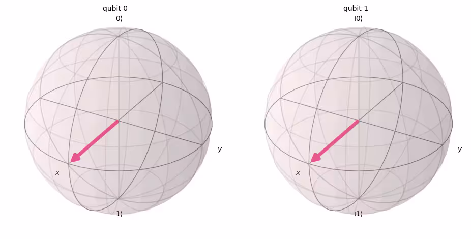
다음 코드를 사용하여 2-Qubit 양자 Circuit을 만들 수 있습니다. 각 Qubit에 H Gate를 적용해 보겠습니다.

# Create the two qubits quantum circuit
qc = QuantumCircuit(2)

# Apply an H gate to qubit 0
qc.h(0)

# Apply an H gate to qubit 1
qc.h(1)

# Draw the circuit
qc.draw(output="mpl")

# See the statevector
out_vector = Statevector(qc)
print(out_vector)

Statevector([0.5+0.j, 0.5+0.j, 0.5+0.j, 0.5+0.j],
            dims=(2, 2))

참고: Qiskit의 비트 순서

Qiskit은 Qubit과 비트의 순서를 나타낼 때 Little Endian 표기법을 사용합니다. 즉, Qubit 0이 비트 문자열에서 가장 오른쪽 비트입니다. 예시: $|01\rangle$은 q0이 $|1\rangle$이고 q1이 $|0\rangle$임을 의미합니다. 양자 컴퓨팅의 일부 문헌에서는 Big Endian 표기법(Qubit 0이 가장 왼쪽 비트)을 사용하며, 양자 역학 문헌에서도 그런 경우가 많으므로 주의하세요.

또한 양자 Circuit을 표현할 때 $|q_0\rangle$은 항상 Circuit의 맨 위에 배치된다는 점도 기억하세요. 이를 염두에 두면, 위 Circuit의 양자 상태는 단일 Qubit 양자 상태의 텐서곱으로 표현할 수 있습니다.

$|q1\rangle \otimes|q0\rangle = (a|0\rangle+b|1\rangle) \otimes (c|0\rangle+d|1\rangle)$

$= ac|0\rangle|0\rangle+ad|0\rangle|1\rangle+bc|1\rangle|0\rangle+bd|1\rangle|1\rangle$

$= ac|00\rangle+ad|01\rangle+bc|10\rangle+bd|11\rangle$

( $|ac|^2+ |ad|^2+ |bc|^2+ |bd|^2=1$ )

Qiskit의 초기 상태는 $|0\rangle|0\rangle=|00\rangle$이므로, 각 Qubit에 $H$를 적용하면 균등한 중첩 상태로 변환됩니다.

$H|0\rangle \otimes H|0\rangle=\frac{1}{\sqrt{2}}(|0\rangle+|1\rangle) \otimes \frac{1}{\sqrt{2}}(|0\rangle+|1\rangle) = \frac{1}{2}(|00\rangle+|01\rangle+|10\rangle+|11\rangle)$

$$=\frac{1}{2}\left( \begin{pmatrix} 1 \\ 1 \end{pmatrix} \otimes \begin{pmatrix} 1 \\ 1 \end{pmatrix}\right) = \frac{1}{2}\begin{pmatrix} 1 \\ 1 \\ 1 \\ 1 \end{pmatrix}=\frac{1}{2}\left(\begin{pmatrix} 1 \\ 0 \\ 0 \\ 0 \end{pmatrix}+\begin{pmatrix} 0 \\ 1 \\ 0 \\ 0 \end{pmatrix}+\begin{pmatrix} 0 \\ 0 \\ 1 \\ 0 \end{pmatrix}+\begin{pmatrix} 0 \\ 0 \\ 0 \\ 1 \end{pmatrix}\right)$$

측정 규칙은 단일 Qubit의 경우와 동일하며, $|00\rangle$을 측정할 확률은 $|ac|^2$입니다.

# Draw a Bloch sphere
plot_bloch_multivector(out_vector)

다음으로, 이 Circuit을 측정해 보겠습니다.

# Create a new circuit with two qubits (first argument) and two classical bits (second argument)
qc = QuantumCircuit(2, 2)

# Apply the gates
qc.h(0)
qc.h(1)

# Add the measurement gates
qc.measure(0, 0)  # Measure qubit 0 and save the result in bit 0
qc.measure(1, 1)  # Measure qubit 1 and save the result in bit 1

# Draw the circuit
qc.draw(output="mpl")

이번에는 Aer 시뮬레이터를 사용하여 모든 가능한 출력 상태의 상대적 확률이 대략 동일한지 실험적으로 검증해 보겠습니다.

# Run the circuit on a simulator to get the results
# Define backend
backend = AerSimulator()

# Transpile to backend
pm = generate_preset_pass_manager(backend=backend, optimization_level=1)
isa_qc = pm.run(qc)

# Run the job
sampler = Sampler(mode=backend)
job = sampler.run([isa_qc])
result = job.result()

# Print the results
counts = result[0].data.c.get_counts()
print(counts)

# Plot the counts in a histogram
plot_histogram(counts)

{'10': 262, '01': 246, '00': 265, '11': 251}

예상대로 $|00\rangle$, $|01\rangle$, $|10\rangle$, $|11\rangle$ 각각이 약 25%의 확률로 측정되었습니다.

4.2 다중 Qubit 양자 Gate

CNOT Gate

CNOT("controlled NOT" 또는 CX) Gate는 2-Qubit Gate로, 제어 Qubit(control qubit)과 표적 Qubit(target qubit)이라는 두 Qubit에 동시에 작용합니다. CNOT은 제어 Qubit이 $|1\rangle$일 때만 표적 Qubit을 반전시킵니다.

입력 (target, control)	출력 (target, control)
00	00
01	11
10	10
11	01

먼저 q0과 q1이 모두 $|0\rangle$인 경우에 이 2-Qubit Gate의 동작을 시뮬레이션하고 출력 상태벡터를 구해 보겠습니다. Qiskit에서 사용하는 문법은 qc.cx(제어 Qubit, 표적 Qubit)입니다.

# Create a circuit with two quantum registers and two classical registers
qc = QuantumCircuit(2, 2)

# Apply the CNOT (cx) gate to a |00> state.
qc.cx(0, 1)  # Here the control is set to q0 and the target is set to q1.

# Draw the circuit
qc.draw(output="mpl")

# See the statevector
out_vector = Statevector(qc)
print(out_vector)

Statevector([1.+0.j, 0.+0.j, 0.+0.j, 0.+0.j],
            dims=(2, 2))

예상대로, 제어 Qubit이 $|0\rangle$ 상태에 있었으므로 $|00\rangle$에 CNOT Gate를 적용해도 상태가 변하지 않았습니다. 이제 CNOT 연산으로 돌아가서, 이번에는 $|01\rangle$에 CNOT Gate를 적용하면 어떻게 되는지 확인해 보겠습니다.

qc = QuantumCircuit(2, 2)

# q0=1, q1=0
qc.x(0)  # Apply a X gate to initialize q0 to 1
qc.cx(0, 1)  # Set the control bit to q0 and the target bit to q1.

# Draw the circuit
qc.draw(output="mpl")

# See the statevector
out_vector = Statevector(qc)
print(out_vector)

Statevector([0.+0.j, 0.+0.j, 0.+0.j, 1.+0.j],
            dims=(2, 2))

CNOT Gate를 적용함으로써 $|01\rangle$ 상태가 $|11\rangle$로 바뀌었습니다.

시뮬레이터에서 Circuit을 실행하여 이 결과를 검증해 보겠습니다.

# Add measurements
qc.measure(0, 0)
qc.measure(1, 1)

# Draw the circuit
qc.draw(output="mpl")

# Run the circuit on a simulator to get the results
# Define backend
backend = AerSimulator()

# Transpile to backend
pm = generate_preset_pass_manager(backend=backend, optimization_level=1)
isa_qc = pm.run(qc)

# Run the job
sampler = Sampler(backend)
job = sampler.run([isa_qc])
result = job.result()

# Print the results
counts = result[0].data.c.get_counts()
print(counts)

# Plot the counts in a histogram
plot_histogram(counts)

{'11': 1024}

결과를 보면 $|11\rangle$이 100%의 확률로 측정된 것을 확인할 수 있습니다.

4.3 양자 얽힘과 실제 양자 장치에서의 실행

먼저 양자 계산에서 특히 중요한 특정 얽힘 상태를 소개한 다음, "얽힘"이라는 용어를 정의하겠습니다.

$$\frac{1}{\sqrt{2}}|00\rangle + \frac{1}{\sqrt{2}}|11\rangle$$

이 상태를 **벨 상태(Bell state)**라고 합니다.

얽힘 상태란, 양자 상태 $|\psi_A\rangle$와 $|\psi_B\rangle$로 구성된 상태 $|\psi_{AB}\rangle$가 개별 양자 상태의 텐서 곱으로 표현될 수 없는 상태를 말합니다.

아래의 $|\psi_{AB}\rangle$가 두 상태 $|\psi\rangle_A$와 $|\psi\rangle_B$를 가진다면,

$$|\psi_{AB}\rangle = \frac{1}{\sqrt{2}}(|00\rangle +|11\rangle) = \frac{1}{\sqrt{2}}(|0\rangle_A|0\rangle_B +|1\rangle_A|1\rangle_B)$$ $$|\psi\rangle_A = a_0|0\rangle+a_1|1\rangle$$ $$|\psi\rangle_B = b_0|0\rangle+b_1|1\rangle$$

이 두 상태의 텐서 곱은 다음과 같습니다.

$$|\psi\rangle _A\otimes |\psi\rangle _B = a_0 b_0|00\rangle+a_0 b_1|01\rangle+a_1 b_0|10\rangle+a_1 b_1|11\rangle$$

그러나 이 두 방정식을 동시에 만족하는 계수 $a_0, a_1, b_0,$ $b_1$은 존재하지 않습니다. 따라서 $|\psi_{AB}\rangle$는 개별 양자 상태인 $|\psi\rangle_A$와 $|\psi\rangle_B$의 텐서 곱으로 표현될 수 없으며, 이는 $|\psi_{AB}\rangle = \frac{1}{\sqrt{2}}(|00\rangle +|11\rangle)$이 얽힘 상태임을 의미합니다.

벨 상태를 만들고 실제 양자 컴퓨터에서 실행해 봅시다. 이제 **Qiskit 패턴(Qiskit patterns)**이라 불리는 양자 프로그램 작성의 네 단계를 따르겠습니다.

1. 문제를 양자 Circuit과 연산자로 변환
2. 목표 하드웨어에 맞게 최적화
3. 목표 하드웨어에서 실행
4. 결과 후처리

Step 1. 문제를 양자 Circuit과 연산자로 변환

양자 프로그램에서 양자 Circuit은 양자 명령을 표현하는 기본 형식입니다. Circuit을 만들 때는 보통 새 QuantumCircuit 객체를 생성한 후 명령을 순서대로 추가합니다.

다음 코드 셀은 앞서 살펴본 특정 두 Qubit 얽힘 상태인 벨 상태를 생성하는 Circuit을 만듭니다.

qc = QuantumCircuit(2, 2)

qc.h(0)
qc.cx(0, 1)

qc.measure(0, 0)
qc.measure(1, 1)

qc.draw("mpl")

Step 2. 목표 하드웨어에 맞게 최적화

Qiskit은 추상적인 Circuit을 목표 하드웨어의 제약을 준수하는 QISA(양자 명령 집합 아키텍처) Circuit으로 변환하고 Circuit 성능을 최적화합니다. 따라서 최적화 전에 목표 하드웨어를 지정해야 합니다. qiskit-ibm-runtime이 설치되어 있지 않다면 먼저 설치해야 합니다. Qiskit Runtime에 대한 자세한 내용은 API 레퍼런스를 참고하세요.

# Install
# !pip install qiskit-ibm-runtime

목표 하드웨어를 지정합니다.

from qiskit_ibm_runtime import QiskitRuntimeService

service = QiskitRuntimeService()
service.backends()

# You can specify the device
# backend = service.backend('ibm_kingston')

# You can also identify the least busy device
backend = service.least_busy(operational=True)
print("The least busy device is ", backend)

Circuit을 트랜스파일(transpile)하는 것은 복잡한 과정입니다. 간단히 말하면, 이 과정은 Circuit을 특정 양자 컴퓨터가 구현할 수 있는 "네이티브 게이트(native gates)"를 사용하는 논리적으로 동등한 Circuit으로 재작성하고, Circuit의 Qubit을 목표 양자 컴퓨터의 최적 실제 Qubit에 매핑합니다. 트랜스파일에 대한 자세한 내용은 이 문서를 참고하세요.

# Transpile the circuit into basis gates executable on the hardware
pm = generate_preset_pass_manager(backend=backend, optimization_level=1)
target_circuit = pm.run(qc)

target_circuit.draw("mpl", idle_wires=False)

트랜스파일 과정에서 Circuit이 새로운 Gate를 사용하도록 재작성된 것을 확인할 수 있습니다. 자세한 내용은 ECRGate 문서를 참고하세요.

Step 3. 목표 Circuit 실행

이제 실제 장치에서 목표 Circuit을 실행합니다.

sampler = Sampler(backend)
job_real = sampler.run([target_circuit])

job_id = job_real.job_id()
print("job id:", job_id)

양자 컴퓨터는 귀중한 자원이며 수요가 매우 높기 때문에, 실제 장치에서의 실행은 큐에서 대기해야 할 수 있습니다. job_id는 나중에 작업의 실행 상태와 결과를 확인하는 데 사용됩니다.

# Check the job status (replace the job id below with your own)
job_real.status(job_id)

IBM Quantum 대시보드에서도 작업 상태를 확인할 수 있습니다：https://quantum.cloud.ibm.com/workloads

# If the Notebook session got disconnected you can also check your job status by running the following code
from qiskit_ibm_runtime import QiskitRuntimeService

service = QiskitRuntimeService()
job_real = service.job(job_id)  # Input your job-id between the quotations
job_real.status()

# Execute after job has successfully run
result_real = job_real.result()
print(result_real[0].data.c.get_counts())

Step 4. 결과 후처리

마지막으로, 값이나 그래프 같은 기대하는 형식의 출력을 생성하기 위해 결과를 후처리해야 합니다.

plot_histogram(result_real[0].data.c.get_counts())

보면 알 수 있듯이, $|00\rangle$과 $|11\rangle$이 가장 자주 관측됩니다. 예상 데이터 외에 몇 가지 다른 결과가 있는데, 이는 노이즈와 Qubit 결맞음 손실(decoherence) 때문입니다. 양자 컴퓨터의 오류와 노이즈에 대해서는 이 과정의 이후 강의에서 더 자세히 배울 것입니다.

4.4 GHZ 상태

얽힘의 개념은 두 Qubit 이상의 시스템으로 확장할 수 있습니다. GHZ 상태(Greenberger-Horne-Zeilinger 상태)는 세 개 이상의 Qubit이 최대로 얽힌 상태입니다. 세 Qubit에 대한 GHZ 상태는 다음과 같이 정의됩니다.

$$\frac{1}{\sqrt 2}(|000\rangle + |111\rangle)$$

이 상태는 다음 양자 Circuit으로 만들 수 있습니다.

qc = QuantumCircuit(3, 3)

qc.h(0)
qc.cx(0, 1)
qc.cx(1, 2)

qc.measure(0, 0)
qc.measure(1, 1)
qc.measure(2, 2)

qc.draw("mpl")

양자 Circuit의 "깊이(depth)"는 Circuit을 설명하는 데 유용하고 널리 쓰이는 지표입니다. Circuit을 왼쪽에서 오른쪽으로 이동하면서 경로를 추적하되, 다중 Qubit Gate로 연결된 경우에만 Qubit을 전환합니다. 해당 경로를 따라 Gate 수를 셉니다. Circuit 내 임의의 경로에서 나타날 수 있는 Gate의 최대 개수가 바로 깊이입니다. 현대의 잡음이 있는 양자 컴퓨터에서는 깊이가 낮은 Circuit일수록 오류가 적고 좋은 결과를 반환할 가능성이 높습니다. 깊이가 매우 깊은 Circuit은 그렇지 않습니다.

QuantumCircuit.depth()를 사용하면 양자 Circuit의 깊이를 확인할 수 있습니다. 위 Circuit의 깊이는 4입니다. 맨 위 Qubit에는 측정을 포함해 세 개의 Gate만 있습니다. 하지만 맨 위 Qubit에서 Qubit 1 또는 Qubit 2로 내려가는 경로에는 CNOT Gate가 하나 더 포함됩니다.

qc.depth()

4

Exercise 2

8-Qubit 시스템의 GHZ 상태는 다음과 같습니다.

$$\frac{1}{\sqrt 2}(|00000000\rangle + |11111111\rangle)$$

이 상태를 가능한 한 얕은 Circuit으로 준비하는 코드를 작성하세요. 측정 Gate를 포함하여 가장 얕은 양자 Circuit의 깊이는 5입니다.

풀이:

# Step 1
qc = QuantumCircuit(8, 8)

##your code goes here##
qc.h(0)
qc.cx(0, 4)
qc.cx(4, 6)
qc.cx(6, 7)

qc.cx(4, 5)

qc.cx(0, 2)
qc.cx(2, 3)

qc.cx(0, 1)
qc.barrier()  # for visual separation

# measure
for i in range(8):
    qc.measure(i, i)

qc.draw("mpl")
# print(qc.depth())

print(qc.depth())

5

from qiskit.visualization import plot_histogram
# Step 2
# For this exercise, the circuit and operators are simple, so no optimizations are needed.

# Step 3
# Run the circuit on a simulator to get the results
backend = AerSimulator()

pm = generate_preset_pass_manager(backend=backend, optimization_level=1)
isa_qc = pm.run(qc)

sampler = Sampler(mode=backend)
job = sampler.run([isa_qc], shots=1024)
result = job.result()

counts = result[0].data.c.get_counts()
print(counts)

# Step 4
# Plot the counts in a histogram

plot_histogram(counts)

{'11111111': 535, '00000000': 489}

5. 요약

여러분은 양자 비트와 Gate를 사용한 Circuit 모델로 양자 계산을 배우고, 중첩, 측정, 얽힘을 복습했습니다. 또한 실제 양자 장치에서 양자 Circuit을 실행하는 방법도 배웠습니다.

GHZ Circuit을 만드는 마지막 연습에서는 Circuit 깊이를 줄이는 방법을 시도했는데, 이는 잡음이 있는 양자 컴퓨터에서 유틸리티 규모의 해법을 얻기 위한 중요한 요소입니다. 이 과정의 이후 강의에서는 잡음과 오류 완화 방법에 대해 자세히 배울 것입니다. 이번 강의에서는 도입부로서 이상적인 장치에서의 Circuit 깊이 줄이기를 다루었지만, 실제로는 Qubit 연결성과 같은 실제 장치의 제약을 고려해야 합니다. 이에 대해서는 이 과정의 이후 강의에서 더 자세히 배울 것입니다.

# See the version of Qiskit
import qiskit

qiskit.__version__

'2.0.2'