노이즈가 있는 양자 프로세서에서 견고하고 결맞은 비아벨 하드론 동역학 관측
사용량 추정치: Heron 프로세서(ibm_boston 또는 동급)에서 6분 (참고: 이는 추정치일 뿐입니다. 실제 실행 시간은 다를 수 있습니다.)
학습 목표
-
효율적인 양자 시뮬레이션을 위해 Loop-String-Hadron(LSH) 프레임워크를 사용하여 비아벨 격자 게이지 이론(특히 SU(2))을 어떻게 재구성할 수 있는지
-
근사적인 SU(2) 게이지 이론 해밀토니안에 대한 Trotter화된 시간 진화 회로를 구축하고 이를 큐비트에 매핑하는 방법
-
판독 오류 완화와 함께 Qiskit Estimator 프리미티브를 사용하여 IBM Quantum® 하드웨어에서 이러한 회로를 실행하는 방법
사전 준비 사항
-
양자장론 개념에 대한 기본적인 친숙함(도움이 되지만 필수는 아님; 배경 섹션에서 필수 사항을 다룹니다)
배경
동기
강력의 SU(3) 게이지 이론인 양자 색역학(QCD)은 쿼크를 하드론으로 결합시키며 가둠(confinement)과 끈 끊김(string breaking)을 지배합니다. 고전적인 격자 QCD 방법은 정적 성질에는 뛰어나지만, 부호 문제(sign problem) 때문에 실시간 동역학을 시뮬레이션할 수 없습니다. 양자 컴퓨터는 게이지 장 자유도를 큐비트에 직접 인코딩함으로써 이 장벽을 우회하는 경로를 제공합니다.
이 튜토리얼은 이러한 시뮬레이션을 시연합니다. IBM Quantum 하드웨어를 사용하여 (1+1)차원 SU(2) 격자 게이지 이론에서 실시간 하드론 전파를 시뮬레이션합니다 — 이는 가장 단순한 비아벨 게이지 이론이며 완전한 QCD로 나아가는 디딤돌입니다.
Kogut-Susskind 해밀토니안
이 이론은 사이트에 스태거드 페르미온(물질)을, 링크에 SU(2) 게이지 장을 갖는 1차원 공간 격자 위에서 정식화됩니다. 무차원 형태로 재척도화한 후 해밀토니안은 다음과 같습니다:
여기서 는 색전기장 에너지, 은 스태거드 질량 항, 는 물질-게이지 상호작용(호핑) 항이며, 는 페르미온 질량을 나타내고, 는 상호작용 세기입니다. 이 이론의 연속체 극한은 이고 일 때 나타납니다.
루프-스트링-하드론(LSH) 프레임워크
핵심 과제는 각 링크의 게이지 장 힐베르트 공간이 무한 차원이라는 점입니다. 루프-스트링-하드론(LSH) 프레임워크는 이론을 게이지 불변 변수 — 플럭스 루프, 분리된 전하를 연결하는 스트링, 그리고 하드론(한 사이트에서의 게이지 단일항 페르미온 쌍) — 로 재정식화하여 이 문제를 해결합니다. LSH 기저에서는 가우스 법칙이 구조적으로 자동으로 만족되므로 모든 기저 상태가 물리적입니다. 각 격자 사이트는 루프 수, 들어오는 스트링, 나가는 스트링을 나타내는 세 개의 양자수 로 특징지어지며, 여기서 은 페르미온성이고 은 보손성입니다. 국소 페르미온 수는 이로부터 짝수 사이트에 대해 로, 홀수 사이트에 대해 로 정의됩니다.
완전한 해밀토니안에서 양자 회로로: 세 가지 핵심 근사
양자 회로는 완전한 SU(2) 해밀토니안을 정확하게 시뮬레이션하지 않습니다. 대신 약결합 영역()에서 유효한 일련의 통제된 근사를 구현합니다. 무엇이 근사되고 무엇이 근사되지 않는지 이해하는 것이 중요합니다:
근사 1 — 에 대한 약결합 극한: 완전한 상호작용 해밀토니안 ([1]의 식 16)에는 과 같은 항을 통해 보손 양자수 에 의존하는 계수들이 포함되어 있습니다. 약결합 영역()에서는 동역학이 큰 을 갖는 상태를 선호하는 전기 항 에 의해 지배됩니다. 인 경우 비율 이 되어 이러한 모든 계수가 1로 단순화됩니다. 그러면 상호작용 해밀토니안은 순전히 국소적인 최근접 이웃 호핑으로 축소됩니다:
이는 과 무관하며 페르미온 큐비트에만 작용합니다.
근사 2 — 에 대한 전역 평균 플럭스: 전기 에너지는 각 링크에서 에 의존합니다. 약결합 진공에서 은 크고 대략 균일합니다. 사이트별 값을 단일 전역 평균 로 대체하면, 는 각 사이트의 페르미온 구성에 비례하는 대각 위상이 됩니다:
여기서 는 페르미온 구성 인 사이트들에 대한 합이며, 는 무시할 수 있는 전역 위상입니다.
근사 3 — Trotter화: 지속 시간 인 한 스텝에 대한 시간 전개 연산자는 다음과 같이 분해됩니다:
여기서 , , 입니다. 이 1차 Trotter 분해는 에 따라 사라지는 오차를 도입합니다. 전체에서 로 고정합니다.
이 세 가지 근사의 결과는 사이트당 두 개의 페르미온 큐비트 만이 동적이라는 것입니다 — 보손 자유도 은 유효 매개변수로 흡수되었습니다. 이는 개의 격자 사이트에 대해 개의 큐비트를 갖는 컴팩트한 회로를 만들어내며, 각 Trotter 스텝은 일정한 2큐비트 게이트 깊이(스텝당 13개)를 갖습니다.
이 튜토리얼에서 시뮬레이션하는 것
이 튜토리얼은 하드론 전파를 시뮬레이션합니다. 강결합 진공(곱 상태)에서 시작하여 격자 중심에 메손을 배치하고 시간에 따라 전개시킵니다. 중앙 메손이 있는 경우와 없는 경우로 회로를 실행한 다음 그 차이를 구하는 차등 측정 프로토콜은 하드웨어 잡음과 경계 효과 모두로부터 결맞은 하드론 신호를 분리합니다. 그 결과는 갇힌 메손 호흡 모드의 특징인 페르미온 밀도 진동의 광원뿔 패턴입니다.
요구 사항
이 튜토리얼을 시작하기 전에 다음을 설치하세요:
-
Qiskit SDK v2.0 이상, 시각화 지원 포함
-
Qiskit Runtime v0.22 이상 (
pip install qiskit-ibm-runtime) -
Pauli Propagation 패키지 (
pip install pauli-prop) -
NumPy (
pip install numpy) -
Matplotlib (
pip install matplotlib)
설정
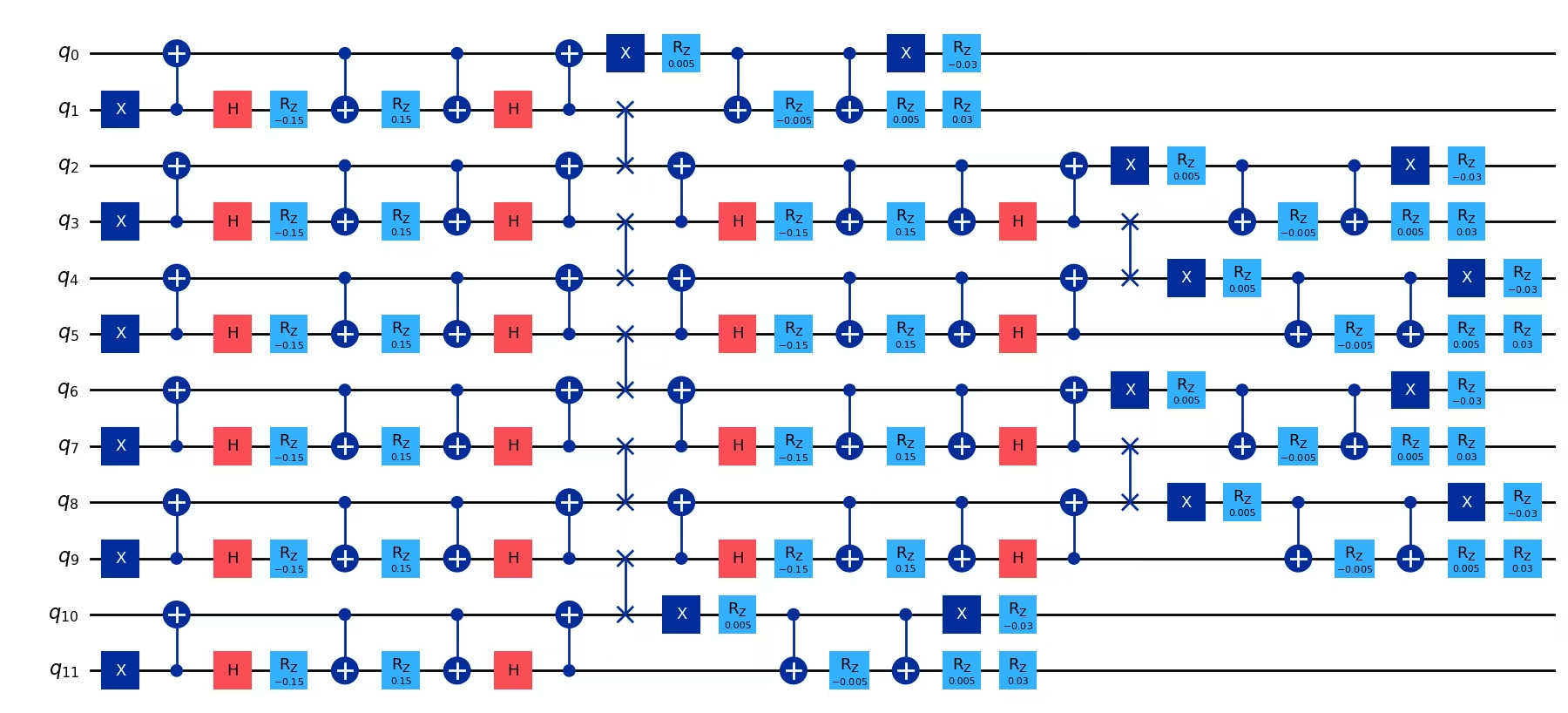
필요한 라이브러리를 가져오고 LSH 시간 전개를 위한 양자 회로를 구축하는 헬퍼 함수를 정의하는 것부터 시작합니다. 회로 구축을 위한 세 가지 핵심 함수가 있습니다:
-
pair_hamiltonian_circuit: 인접 사이트 간의 근사 상호작용 해밀토니안에 대한 2큐비트 유니터리 를 구현합니다. 게이트 분해는 다음과 같습니다: . -
electric_hamiltonian_circuit: 각 사이트에서의 근사 전기장 에너지에 대한 2큐비트 유니터리 를 구현합니다. 게이트 분해는 다음과 같습니다: . -
construct_circuit: 큐비트 연결성을 관리하기 위한 SWAP 게이트와 함께 상호작용, 전기, 질량 항을 층층이 쌓아 전체 Trotter화된 회로를 조립합니다.
# Added by doQumentation — required packages for this notebook
!pip install -q matplotlib numpy pauli-prop qiskit qiskit-ibm-runtime
# Import libraries

import numpy as np
import matplotlib.pyplot as plt
from matplotlib.colors import TwoSlopeNorm
from qiskit.circuit import QuantumCircuit
from qiskit.quantum_info import SparsePauliOp
from typing import Optional

import warnings

warnings.filterwarnings("ignore")
def pair_hamiltonian_circuit(c: float) -> QuantumCircuit:
    """Two-qubit unitary for the approximate interaction Hamiltonian H_I.

    Implements exp(-i * c * H_I^approx) for one pair of neighboring sites,
    where c = delta_tau * x.
    """
    qc_temp = QuantumCircuit(2)
    qc_temp.cx(1, 0)
    qc_temp.h(1)
    qc_temp.rz(-c, 1)
    qc_temp.cx(0, 1)
    qc_temp.rz(c, 1)
    qc_temp.cx(0, 1)
    qc_temp.h(1)
    qc_temp.cx(1, 0)
    return qc_temp

def electric_hamiltonian_circuit(theta: float) -> QuantumCircuit:
    """Two-qubit unitary for the approximate electric field Hamiltonian H_E.

    Implements exp(-i * theta * H_E^approx) for one lattice site,
    where theta = -delta_tau * (n_bar_l / 2 + 3/4).
    """
    qc_temp = QuantumCircuit(2)
    qc_temp.x(0)
    qc_temp.rz(theta / 2, 0)
    qc_temp.cx(0, 1)
    qc_temp.rz(-theta / 2, 1)
    qc_temp.cx(0, 1)
    qc_temp.rz(theta / 2, 1)
    qc_temp.x(0)
    return qc_temp

def construct_circuit(
    num_lattice_point: int,
    num_trotter_steps: int,
    c: float,
    theta: float,
    m: float,
    theory: Optional[int] = 2,
    barriers: Optional[bool] = False,
    measurement: Optional[bool] = False,
    add_init_state: Optional[bool] = True,
    inverse_mid: Optional[bool] = False,
) -> QuantumCircuit:
    """Construct the full Trotterized time-evolution circuit.

    Builds a circuit implementing n Trotter steps of the approximate SU(2)
    LSH Hamiltonian evolution. The qubit layout uses a zigzag ordering:
    n_i(0), n_i(1), n_o(0), n_o(1), n_i(2), n_i(3), n_o(2), n_o(3), ...
    which minimizes the number of SWAP layers needed.

    Args:
        num_lattice_point: Number of lattice sites
        (num_qubits = 2 * num_lattice_point).
        num_trotter_steps: Number of Trotter steps.
        c: Interaction parameter (delta_tau * x).
        theta: Electric field phase parameter.
        m: Mass parameter (m_tilde = delta_tau * mu).
        theory: 1 for single chain, 2 for SU(2). Default 2.
        barriers: Insert barriers between Trotter layers for
        visualization.
        measurement: Append measurements at the end.
        add_init_state: Prepare the half-filled (strong-coupling vacuum)
        initial state.
        inverse_mid: Swap the central sites
        (for differential measurement protocol).
    """
    num_qubits = theory * num_lattice_point
    qc = QuantumCircuit(num_qubits)

    if num_trotter_steps <= 0:
        return qc

    # --- Initial state preparation ---
    if add_init_state:
        i = 1
        while i < num_lattice_point:
            for j in range(theory):
                qc.x(i + j * num_lattice_point)
            i = i + 2
        if inverse_mid:
            mid_lattice_qubits = [num_qubits // 2 - 1, num_qubits // 2]
            qc.x(mid_lattice_qubits)
    else:
        i = 1
        while i < num_qubits - 1:
            qc.swap(i, i + 1)
            i = i + 4

    # --- Trotter steps ---
    for step in range(num_trotter_steps):
        if barriers:
            qc.barrier()

        # First SWAP layer (skipped at step 0 — absorbed into initial state mapping)
        if step > 0:
            i = 1
            while i < num_qubits - 1:
                qc.swap(i, i + 1)
                i = i + 4

        # First layer of pair interactions
        j = 0
        while j < num_qubits - 2:
            circ = pair_hamiltonian_circuit(c)
            qc.compose(circ, [j, j + 1], inplace=True)
            j = j + 2
        if num_lattice_point % 2 == 0:
            circ = pair_hamiltonian_circuit(c)
            qc.compose(circ, [j, j + 1], inplace=True)

        # Second SWAP layer
        i = 1
        while i < num_qubits - 1:
            qc.swap(i, i + 1)
            i = i + theory

        # Second layer of pair interactions
        j = 2
        while j < num_qubits - 3:
            circ = pair_hamiltonian_circuit(c)
            qc.compose(circ, [j, j + 1], inplace=True)
            j = j + 2
        if num_lattice_point % 2 != 0:
            circ = pair_hamiltonian_circuit(c)
            qc.compose(circ, [j, j + 1], inplace=True)

        # Third SWAP layer
        i = 3
        while i < num_qubits - 1:
            qc.swap(i, i + 1)
            i = i + 2 * theory

        # Electric field term
        if theta != 0:
            e_circ = electric_hamiltonian_circuit(theta)
            for j in range(num_lattice_point):
                qc.compose(e_circ, [2 * j, 2 * j + 1], inplace=True)

        # Mass term: Rz(-m_tilde) for even sites, Rz(m_tilde) for odd sites
        for q in range(num_qubits):
            if q % 2 == 0:
                qc.rz(-1 * m, q)
            else:
                qc.rz(m, q)

    if measurement:
        qc.measure_all()

    return qc
def get_probabilities(expval: float):
    """Convert a Z-expectation value to site occupation probability.

    Since <Z> = p(0) - p(1), the occupation probability is p(1) = (1 - <Z>) / 2.
    """
    p1 = round((1 - expval) / 2, 3)
    return p1

def get_number(expval_data, num_lattice_point):
    """Convert raw Z-expectation values to staggered fermion number n_f at each site.

    n_f(r) = n_i(r) + n_o(r)           for even r
    n_f(r) = 2 - [n_i(r) + n_o(r)]     for odd r

    The two qubits per site encode (n_i, n_o), and occupation probabilities
    give us <n_i> and <n_o>.
    """
    N = []
    for expvals in expval_data:
        Pstep = [get_probabilities(expval) for expval in expvals]
        Nstep = []
        for k in range(num_lattice_point):
            val = Pstep[2 * k] + Pstep[2 * k + 1]
            a = 2 * (k % 2) + (1 - 2 * (k % 2)) * val
            Nstep.append(float(a))
        N.append(Nstep)
    return N

def calculate_difference(N, N_mid, num_lattice_point):
    """Differential measurement protocol: |n_f(meson) - n_f(vacuum)|.

    Subtracting the vacuum (SCV) evolution from the meson evolution
    isolates the coherent hadron signal from symmetric noise and boundary effects.
    """
    N_diff = []
    for i in range(len(N)):
        Nstep_diff = []
        for j in range(num_lattice_point):
            Nstep_diff.append(abs(N[i][j] - N_mid[i][j]))
        N_diff.append(Nstep_diff)
    return N_diff
소규모 시뮬레이터 예제
먼저 6개 사이트 격자(12큐비트)를 사용하여 소규모로 워크플로를 시연함으로써, 하드웨어에서 실행하기 전에 회로 구성을 검증하고 물리적 관측량을 이해할 수 있도록 합니다.
1단계: 고전적 입력을 양자 문제로 매핑하기
논문에서 연구된 약결합 영역과 일치하는 물리적 매개변수(, )를 정의합니다. 유도된 회로 매개변수는 다음과 같습니다:
-
(상호작용 매개변수)
-
(전기장 위상)
-
(질량 매개변수)
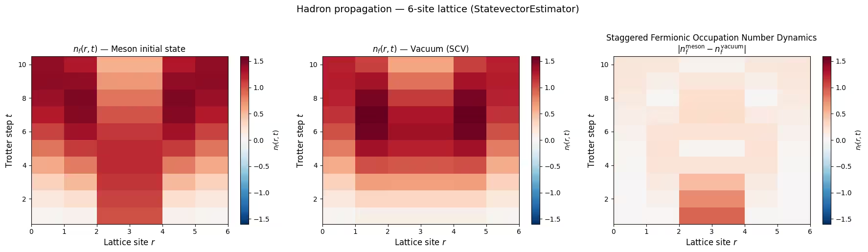
각 Trotter 스텝 수에 대해 두 개의 회로를 구축합니다: 중심에 메손을 초기화하는 회로(inverse_mid=True)와 강결합 진공을 준비하는 회로(inverse_mid=False)입니다. 차등 측정 프로토콜은 하드론 신호를 분리하기 위해 진공 전개를 뺍니다.
# Physical / circuit parameters
num_lattice_point = 6  # 6 lattice sites -> 12 qubits for SU(2)
num_qubits = 2 * num_lattice_point
c = 0.15  # delta_tau * x
theta = 0.01  # electric field phase
m = 0.03  # m_tilde = delta_tau * mu
trotter_steps = range(1, 11)  # 10 Trotter steps

print(f"Lattice sites: {num_lattice_point}, Qubits: {num_qubits}")
print(f"Parameters: c={c}, theta={theta}, m_tilde={m}")
Lattice sites: 6, Qubits: 12
Parameters: c=0.15, theta=0.01, m_tilde=0.03
# Build circuits: meson initial state and vacuum (SCV) initial state
circuits_mid = [
    construct_circuit(
        num_lattice_point,
        d,
        c,
        theta,
        m,
        barriers=False,
        measurement=False,
        add_init_state=True,
        inverse_mid=True,
    )
    for d in trotter_steps
]

circuits = [
    construct_circuit(
        num_lattice_point,
        d,
        c,
        theta,
        m,
        barriers=False,
        measurement=False,
        add_init_state=True,
        inverse_mid=False,
    )
    for d in trotter_steps
]

# Visualize a single Trotter step
print(
    f"Circuit for 1 Trotter step: {circuits[0].num_qubits} qubits, depth {circuits[0].depth()}"
)
circuits[0].draw("mpl", fold=-1)
Circuit for 1 Trotter step: 12 qubits, depth 26
2단계: 양자 하드웨어 실행을 위한 문제 최적화
관측량을 정의합니다: 모든 큐비트에 대한 단일 큐비트 측정입니다. 로부터 점유 확률을 추출한 다음 각 격자 사이트 에서의 스태거드 페르미온 수 를 구할 수 있습니다.
# Z observable on each qubit
observables = [
    SparsePauliOp("I" * i + "Z" + "I" * (num_qubits - i - 1))
    for i in range(num_qubits)
]

print(f"Number of observables: {len(observables)}")
Number of observables: 12
3단계: Qiskit 프리미티브를 사용하여 실행하기
소규모에서 정확한 노이즈 없는 시뮬레이션을 위해 StatevectorEstimator를 사용합니다.
from qiskit.primitives import StatevectorEstimator

estimator = StatevectorEstimator()

# Run meson circuits
pubs_mid = [(circuit, observables) for circuit in circuits_mid]
result_mid = estimator.run(pubs_mid).result()

# Run vacuum (SCV) circuits
pubs = [(circuit, observables) for circuit in circuits]
result = estimator.run(pubs).result()

# Extract expectation values
raw_expvals_mid = [
    result_mid[i].data.evs[::-1] for i in range(len(circuits_mid))
]
raw_expvals = [result[i].data.evs[::-1] for i in range(len(circuits))]

print(f"Computed expectation values for {len(raw_expvals)} Trotter steps")
Computed expectation values for 10 Trotter steps
4단계: 후처리 후 원하는 고전적 형식으로 결과 반환하기
기댓값을 스태거드 페르미온 수 로 변환하고 차등 측정 프로토콜(메손 진공)을 적용하여 하드론 전파 히트맵을 생성합니다. 이는 참조 논문의 그림 3 구조를 재현합니다: x축에 격자 사이트 , y축에 Trotter 스텝(시간) , 색상 스케일로 를 나타냅니다.
# Compute fermion numbers
N_mid_sim = get_number(raw_expvals_mid, num_lattice_point)
N_sim = get_number(raw_expvals, num_lattice_point)
N_diff_sim = calculate_difference(N_mid_sim, N_sim, num_lattice_point)

# --- Reproduce Figure 3 style: Staggered Fermionic Occupation Number Dynamics ---
fig, axes = plt.subplots(1, 3, figsize=(18, 5))

# Convert to numpy arrays for plotting
N_mid_arr = np.array(N_mid_sim)
N_arr = np.array(N_sim)
N_diff_arr = np.array(N_diff_sim)

# Color scheme
vmax = max(max(sublist) for sublist in N_arr)
vmin = -vmax

# Meson evolution
norm1 = TwoSlopeNorm(vmin=vmin, vcenter=0, vmax=vmax)
im0 = axes[0].imshow(
    N_mid_arr,
    aspect="auto",
    origin="lower",
    cmap="RdBu_r",
    norm=norm1,
    extent=[0, num_lattice_point, 0.5, len(trotter_steps) + 0.5],
)
axes[0].set_xlabel("Lattice site $r$", fontsize=12)
axes[0].set_ylabel("Trotter step $t$", fontsize=12)
axes[0].set_title("$n_f(r,t)$ — Meson initial state", fontsize=12)
plt.colorbar(im0, ax=axes[0], label="$n_f(r,t)$")

# Vacuum (SCV) evolution
im1 = axes[1].imshow(
    N_arr,
    aspect="auto",
    origin="lower",
    cmap="RdBu_r",
    norm=norm1,
    extent=[0, num_lattice_point, 0.5, len(trotter_steps) + 0.5],
)
axes[1].set_xlabel("Lattice site $r$", fontsize=12)
axes[1].set_ylabel("Trotter step $t$", fontsize=12)
axes[1].set_title("$n_f(r,t)$ — Vacuum (SCV)", fontsize=12)
plt.colorbar(im1, ax=axes[1], label="$n_f(r,t)$")

# Differential: meson - vacuum
norm2 = TwoSlopeNorm(vmin=vmin, vcenter=0, vmax=vmax)
im2 = axes[2].imshow(
    N_diff_arr,
    aspect="auto",
    origin="lower",
    cmap="RdBu_r",
    norm=norm2,
    extent=[0, num_lattice_point, 0.5, len(trotter_steps) + 0.5],
)
axes[2].set_xlabel("Lattice site $r$", fontsize=12)
axes[2].set_ylabel("Trotter step $t$", fontsize=12)
axes[2].set_title(
    "Staggered Fermionic Occupation Number Dynamics\n$|n_f^{\\mathrm{meson}} - n_f^{\\mathrm{vacuum}}|$",
    fontsize=12,
)
plt.colorbar(im2, ax=axes[2], label="$n_f(r,t)$")

plt.suptitle(
    f"Hadron propagation — {num_lattice_point}-site lattice (StatevectorEstimator)",
    fontsize=14,
    y=1.02,
)
plt.tight_layout()
plt.show()
대규모 하드웨어 예제
이제 IBM Quantum 하드웨어에서 30개 사이트 격자(60큐비트)로 규모를 확장합니다. 이 규모에서 10개의 Trotter 스텝을 가진 회로는 3400개 이상의 2큐비트 게이트와 14,000개의 단일 큐비트 게이트로 구성됩니다.
1~4단계(단일 코드 블록으로 압축)
하드웨어 워크플로의 핵심 측면:
-
메손 및 진공 회로에 대한 10개의 Trotter 스텝(드리프트를 최소화하기 위해 교차 배치)
-
optimization_level=1로 트랜스파일 — 회로 레이아웃이 이미 장치 토폴로지(선형 체인)와 동형이므로 라우팅 SWAP이 필요하지 않습니다. 트랜스파일러는 저잡음 물리적 큐비트 체인을 선택하고 게이트를 네이티브 게이트 세트로 분해하는 데에만 사용됩니다. -
TREX 판독 오류 완화 및 Pauli 트와일링을 사용하는
EstimatorV2 -
모든 작업을 함께 제출하기 위한
Batch세션
# -------------------------Step 1: Define parameters & build circuits-------------------------

from qiskit_ibm_runtime import QiskitRuntimeService
from qiskit.transpiler.preset_passmanagers import generate_preset_pass_manager
from qiskit_ibm_runtime import EstimatorV2, Batch
from qiskit_ibm_runtime.options import (
    EstimatorOptions,
    ResilienceOptionsV2,
    TwirlingOptions,
    DynamicalDecouplingOptions,
)

service = QiskitRuntimeService()

num_lattice_point_hw = 30
num_qubits_hw = 2 * num_lattice_point_hw  # 60 qubits
c_hw = 0.15
theta_hw = 0.01
m_hw = 0.03
trotter_steps_hw = range(1, 11)  # 10 Trotter steps

# Build meson and vacuum circuits
circuits_mid_hw = [
    construct_circuit(
        num_lattice_point_hw,
        d,
        c_hw,
        theta_hw,
        m_hw,
        barriers=False,
        measurement=False,
        add_init_state=True,
        inverse_mid=True,
    )
    for d in trotter_steps_hw
]

circuits_hw = [
    construct_circuit(
        num_lattice_point_hw,
        d,
        c_hw,
        theta_hw,
        m_hw,
        barriers=False,
        measurement=False,
        add_init_state=True,
        inverse_mid=False,
    )
    for d in trotter_steps_hw
]

print(f"Built {len(circuits_hw)} circuit pairs for {num_qubits_hw} qubits")

# -------------------------Step 2: Transpile for hardware-------------------------
# The circuit topology is a linear chain, isomorphic to the device topology.
# We use optimization_level=1 since no routing SWAPs are needed — the transpiler
# only needs to select a low-noise qubit chain and decompose to native gates.

backend = service.backend("ibm_boston")

layout = [
    140,
    141,
    142,
    143,
    136,
    123,
    122,
    121,
    116,
    101,
    102,
    103,
    96,
    83,
    82,
    81,
    76,
    61,
    62,
    63,
    64,
    65,
    66,
    67,
    68,
    69,
    78,
    89,
    88,
    87,
    97,
    107,
    106,
    105,
    117,
    125,
    126,
    127,
    137,
    147,
    148,
    149,
    150,
    151,
    152,
    153,
    154,
    155,
    139,
    135,
    134,
    133,
    132,
    131,
    130,
    129,
    118,
    109,
    110,
    111,
]

pm = generate_preset_pass_manager(
    optimization_level=1, backend=backend, initial_layout=layout
)

isa_circuits_mid = pm.run(circuits_mid_hw)
isa_circuits = pm.run(circuits_hw)

print(f"Transpiled circuits. Example depth: {isa_circuits[0].depth()}")

# Define and layout-map observables
observables_hw = [
    SparsePauliOp("I" * i + "Z" + "I" * (num_qubits_hw - i - 1))
    for i in range(num_qubits_hw)
]

isa_observables_mid = [
    [obs.apply_layout(isa_circuits_mid[i].layout) for obs in observables_hw]
    for i in range(len(isa_circuits_mid))
]
isa_observables = [
    [obs.apply_layout(isa_circuits[i].layout) for obs in observables_hw]
    for i in range(len(isa_circuits))
]

# Build PUBs — interleave meson and vacuum for each Trotter step
isa_pubs_mid = [
    (circ, obs) for circ, obs in zip(isa_circuits_mid, isa_observables_mid)
]
isa_pubs = [(circ, obs) for circ, obs in zip(isa_circuits, isa_observables)]

pubs_to_execute = [
    [isa_pubs_mid[i], isa_pubs[i]] for i in range(len(isa_pubs))
]

# -------------------------Step 3: Execute on hardware-------------------------

twirling_options = TwirlingOptions(
    enable_gates=True,
    enable_measure=True,
    shots_per_randomization="auto",
    strategy="active-circuit",
)

resilience_options = ResilienceOptionsV2(
    measure_mitigation=True,  # TREX readout error mitigation
    zne_mitigation=False,  # ZNE turned off
)

dd_options = DynamicalDecouplingOptions(
    enable=False  # Circuit is sufficiently dense
)

options = EstimatorOptions(
    resilience=resilience_options,
    twirling=twirling_options,
    dynamical_decoupling=dd_options,
    default_shots=10_000,
)

ids = []
with Batch(backend=backend) as batch:
    for idx, pub in enumerate(pubs_to_execute):
        print(f"Submitting job for Trotter step {idx + 1}")
        estimator = EstimatorV2(mode=batch, options=options)
        estimator.skip_transpilation = True
        job = estimator.run(pub)
        ids.append(job.job_id())
    batch_id = batch.session_id

job_info = {"ids": ids, "batch_id": batch_id}
print(f"Submitted {len(ids)} jobs. Batch ID: {batch_id}")
print(ids)
# -------------------------Step 4: Post-process results-------------------------

jobs = [service.job(job_id) for job_id in ids]
results = [job.result() for job in jobs]

# Extract expectation values (index 0 = meson, index 1 = vacuum)
raw_expvals_mid_hw = [result[0].data.evs[::-1] for result in results]
raw_expvals_hw = [result[1].data.evs[::-1] for result in results]

# Compute fermion numbers and differential
N_mid_hw = get_number(raw_expvals_mid_hw, num_lattice_point_hw)
N_hw = get_number(raw_expvals_hw, num_lattice_point_hw)
N_diff_hw = calculate_difference(N_mid_hw, N_hw, num_lattice_point_hw)
N_diff_hw_arr = np.array(N_diff_hw)

fig, ax = plt.subplots(figsize=(10, 6))
vmax = np.abs(N_hw).max()
vmin = -vmax
norm = TwoSlopeNorm(vmin=vmin, vcenter=0, vmax=vmax)
im = ax.imshow(
    N_diff_hw_arr,
    aspect="auto",
    origin="lower",
    cmap="RdBu_r",
    norm=norm,
    extent=[0, 8, 0.5, len(trotter_steps_hw) + 0.5],
)
ax.set_xlabel("Lattice site $r$", fontsize=13)
ax.set_ylabel("Trotter step $t$", fontsize=13)
ax.set_title(
    "Staggered Fermionic Occupation Number Dynamics\nQuantum Simulation on IBM Hardware — 30-site lattice (60 qubits)",
    fontsize=13,
)
cbar = plt.colorbar(im, ax=ax)
cbar.set_label("$n_f(r,t)$", fontsize=12)
plt.tight_layout()
plt.show()

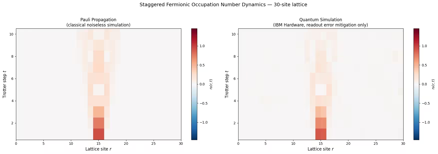
Pauli Propagation을 통한 고전적 벤치마킹
Pauli Propagation Method(PPM)는 하이젠베르크 그림에서 측정된 관측량을 회로를 통해 역전파하여 양자 회로의 노이즈 없는 고전적 시뮬레이션을 제공합니다. 클리포드 레이어(CNOT, H, S, X 게이트) 아래에서 Pauli 연산자는 항의 수를 늘리지 않고 다른 Pauli 연산자로 매핑됩니다. 비클리포드 레이어(회로의 게이트)는 분기를 유발할 수 있으며 — 최악의 경우 항의 수가 두 배가 됩니다 — 그러나 많은 분기는 계수가 작아서 잘라낼 수 있습니다.
pauli-prop를 사용한 워크플로는 다음과 같습니다:
-
evolve_through_cliffords를 사용하여 회로를 클리포드 부분과 비클리포드 부분으로 분할합니다. -
propagate_through_circuit를 사용하여 각 관측량을 비클리포드 부분을 통해 전파하며, 최대max_terms개의 Pauli 항을 유지하고 잘라내기 임계값atol미만의 계수를 갖는 항은 버립니다. -
Qiskit의 내장 클리포드 지원을 사용하여 결과를 클리포드 부분을 통해 전개합니다.
-
대각 Pauli 항(와 만 포함)의 계수를 합산하여 기댓값을 추출합니다.
잘라내기 임계값
propagate_through_circuit의 atol 매개변수는 작은 Pauli 분기가 얼마나 공격적으로 잘려나가는지를 제어합니다. 매우 엄격한 임계값(예: 1e-12)은 거의 모든 분기를 유지하고 정확한 결과를 제공하지만, 시뮬레이션 시간은 회로 깊이에 따라 가파르게 증가합니다. 논문의 120큐비트 시뮬레이션은 기본 설정으로 약 8.5시간이 걸렸습니다. 임계값을 높이면(예: 1e-6 또는 1e-3) 해당 값보다 작은 계수를 갖는 항이 폐기되어 추적되는 항의 수가 크게 줄고 계산 속도가 빨라집니다. 그 대가는 서로 다른 임계값에서의 결과를 비교하여 검증할 수 있는 작고 제어 가능한 근사 오차입니다.
import time
from pauli_prop import evolve_through_cliffords, propagate_through_circuit

# ── PPM Configuration ──
# Truncation threshold: controls the speed/accuracy trade-off.
PPM_THRESHOLD = 1e-3

# Maximum Pauli terms to track per observable (hard cap on memory/time)
PPM_MAX_TERMS = 66_000

print(f"PPM settings: atol={PPM_THRESHOLD}, max_terms={PPM_MAX_TERMS}")

# We propagate each single-qubit Z observable through each circuit.
# For PPM, we work with the un-transpiled circuits (ideal noiseless simulation).

observables_pp = [
    SparsePauliOp("I" * i + "Z" + "I" * (num_qubits_hw - i - 1))
    for i in range(num_qubits_hw)
]

def ppm_expectation_values(
    circuit, observables, max_terms=PPM_MAX_TERMS, atol=PPM_THRESHOLD
):
    """Compute expectation values of single-qubit Z observables
    via Pauli propagation.

    Args:
        circuit: The quantum circuit to simulate.
        observables: List of single-qubit Z observables.
        max_terms: Maximum number of Pauli terms to retain (hard cap).
        atol: Absolute tolerance — Pauli terms with coefficients below this
              value are discarded during propagation. Larger values give
              faster simulation at the cost of approximation accuracy.
    """
    circuit = circuit.decompose(["swap"])  # decompose SWAPs into 3 CX gates
    cliff, non_cliff = evolve_through_cliffords(circuit)

    evs = []
    for obs in observables:
        evolved_obs = propagate_through_circuit(
            obs, non_cliff, max_terms=max_terms, atol=atol, frame="h"
        )[0]
        evolved_obs.paulis = evolved_obs.paulis.evolve(cliff, frame="h")
        diagonal_mask = ~evolved_obs.paulis.x.any(axis=1)
        ev = float(evolved_obs.coeffs[diagonal_mask].sum().real)
        evs.append(ev)
    return np.array(evs)

# Run PPM for each Trotter step and record wall-clock time
pp_expvals_mid = []
pp_expvals = []
pp_times = []

for idx, d in enumerate(trotter_steps_hw):
    t_start = time.perf_counter()

    # Meson circuit
    evs_mid = ppm_expectation_values(circuits_mid_hw[idx], observables_pp)

    # Vacuum circuit
    evs_vac = ppm_expectation_values(circuits_hw[idx], observables_pp)

    elapsed = time.perf_counter() - t_start
    pp_times.append(elapsed)

    pp_expvals_mid.append(evs_mid[::-1])
    pp_expvals.append(evs_vac[::-1])

    print(f"Trotter step {d:2d}: {elapsed:.1f} s")

print(f"\nTotal PPM simulation time: {sum(pp_times):.1f} s")
print(f"Truncation threshold used: {PPM_THRESHOLD}")
PPM settings: atol=0.001, max_terms=66000
Trotter step  1: 5.0 s
Trotter step  2: 7.5 s
Trotter step  3: 11.2 s
Trotter step  4: 14.7 s
Trotter step  5: 18.3 s
Trotter step  6: 22.1 s
Trotter step  7: 25.6 s
Trotter step  8: 29.4 s
Trotter step  9: 33.2 s
Trotter step 10: 36.6 s

Total PPM simulation time: 203.6 s
Truncation threshold used: 0.001
# --- PPM simulation time vs. Trotter steps ---
fig, ax = plt.subplots(figsize=(8, 5))
ax.plot(
    list(trotter_steps_hw),
    pp_times,
    "o-",
    color="tab:blue",
    linewidth=2,
    markersize=6,
)
ax.set_xlabel("Trotter step", fontsize=13)
ax.set_ylabel("Wall-clock time (s)", fontsize=13)
ax.set_title(
    "Pauli Propagation simulation time vs. Trotter steps\n(30-site lattice, 60 qubits)",
    fontsize=13,
)
ax.grid(True, alpha=0.3)
plt.tight_layout()
plt.show()

# --- PPM heatmap and comparison with hardware ---
N_mid_pp = get_number(pp_expvals_mid, num_lattice_point_hw)
N_pp = get_number(pp_expvals, num_lattice_point_hw)
N_diff_pp = calculate_difference(N_mid_pp, N_pp, num_lattice_point_hw)

N_diff_pp_arr = np.array(N_diff_pp)

fig, axes = plt.subplots(1, 2, figsize=(18, 6))
vmax = np.abs(N_hw).max()
vmin = -vmax
norm = TwoSlopeNorm(vmin=vmin, vcenter=0, vmax=vmax)

# PPM result
im0 = axes[0].imshow(
    N_diff_pp_arr,
    aspect="auto",
    origin="lower",
    cmap="RdBu_r",
    norm=norm,
    extent=[0, num_lattice_point_hw, 0.5, len(trotter_steps_hw) + 0.5],
)
axes[0].set_xlabel("Lattice site $r$", fontsize=12)
axes[0].set_ylabel("Trotter step $t$", fontsize=12)
axes[0].set_title(
    "Pauli Propagation\n(classical noiseless simulation)", fontsize=12
)
plt.colorbar(im0, ax=axes[0], label="$n_f(r,t)$")

# Hardware result
im1 = axes[1].imshow(
    N_diff_hw_arr,
    aspect="auto",
    origin="lower",
    cmap="RdBu_r",
    norm=norm,
    extent=[0, num_lattice_point_hw, 0.5, len(trotter_steps_hw) + 0.5],
)
axes[1].set_xlabel("Lattice site $r$", fontsize=12)
axes[1].set_ylabel("Trotter step $t$", fontsize=12)
axes[1].set_title(
    "Quantum Simulation\n(IBM Hardware, readout error mitigation only)",
    fontsize=12,
)
plt.colorbar(im1, ax=axes[1], label="$n_f(r,t)$")

plt.suptitle(
    "Staggered Fermionic Occupation Number Dynamics — 30-site lattice",
    fontsize=14,
    y=1.02,
)
plt.tight_layout()
plt.show()
다음 단계
이 작업이 흥미로웠다면 다음 자료를 살펴보세요:
-
Qiskit Estimator 프리미티브 문서 — 오류 완화 옵션 구성에 대한 세부 정보
-
오류 완화 및 억제 기법 — TREX, ZNE 및 기타 완화 방법에 대해 알아보기
-
Qiskit Pauli Propagation (pauli-prop) — Pauli 역전파를 통한 Rust 가속 고전적 시뮬레이션
참고 문헌
[1] 원 논문: Ilčić, Majumdar, Mathew 외. "Observation of Robust and Coherent Non-Abelian Hadron Dynamics on Noisy Quantum Processors" arXiv:2602.18080 (2026)