Samplex 입력과 출력

소개

Samplex는 samplomatic 라이브러리의 핵심 타입입니다. samplex는 어떤 템플릿 회로의 매개변수에 대한 매개변수화된 확률 분포를 나타내며, 바인딩된 템플릿 회로를 실행하여 수집한 데이터를 후처리할 때 사용할 다른 배열 값 필드도 함께 갖습니다. 핵심 인터페이스는 이 분포에서 샘플을 추출해 배열 모음을 만드는 sample() 메서드입니다.

이 가이드는 sample() 인터페이스를 사용하는 방법, 필요한 입력을 조회하고 지정하는 방법, 예상되는 출력을 확인하는 방법을 설명합니다. sample()에 전달되고 반환되는 배열은 강한 타입을 갖습니다. 즉, samplex 인스턴스에서 배열의 이름, 타입, 형태는 고정되어 있으며 샘플링을 하기 전에 조회할 수 있습니다. samplex에 존재하는 입력과 출력은 여러 요인에 따라 달라집니다. 예를 들어 측정 트윌링이 있는지, 노이즈 주입이 필요한지에 따라 달라집니다. 이러한 이유로 일반적으로 두 samplex 인스턴스가 같은 입력과 출력을 갖는다고 기대할 수 없습니다.

설정

먼저 박스로 묶인 회로를 구성하고 이를 samplex와 템플릿 쌍으로 빌드합니다. 이들은 이어지는 예제에서 사용됩니다. 회로를 수동으로 박스로 묶을 때 이 가이드는 alpha, beta, ref1, ref2, mod_ref1, mod_ref2, mod_ref3, conclude라는 이름을 사용합니다. 또한 이 회로에는 Parameter 객체가 네 개 있습니다. 이 가이드는 이들이 samplex 입력과 출력에서 각각 어떤 역할을 하는지 보여 줍니다. 회로를 자동으로 박스로 묶는 방법은 트랜스파일러 가이드를 참조하세요.

import matplotlib.pyplot as plt
import numpy as np
from qiskit.circuit import ClassicalRegister, Parameter, QuantumCircuit, QuantumRegister
from qiskit.quantum_info import Operator, Pauli, PauliLindbladMap

from samplomatic import ChangeBasis, InjectNoise, Twirl, build

# our circuit has two classical registers named alpha and beta
circuit = QuantumCircuit(
    QuantumRegister(4), alpha := ClassicalRegister(3, "alpha"), beta := ClassicalRegister(1, "beta")
)

# the first box is only twirled
with circuit.box([Twirl()]):
    for idx in range(4):
        circuit.rx(Parameter(f"a{idx}"), idx)
    circuit.cz(0, 1)
    circuit.cz(1, 2)

# the second box is twirled, and has noise injected
with circuit.box([Twirl(), InjectNoise(ref="ref1", modifier_ref="mod_ref1")]):
    circuit.h(1)
    circuit.cz(1, 2)

# the third box is twirled, and has different noise injected
with circuit.box([Twirl(), InjectNoise(ref="ref2", modifier_ref="mod_ref2")]):
    circuit.rx(0.1, range(4))
    circuit.cz(0, 1)
    circuit.cz(1, 2)

# the fourth box is the same as the second, but with a different modifer ref
with circuit.box([Twirl(), InjectNoise(ref="ref1", modifier_ref="mod_ref3")]):
    circuit.h(1)
    circuit.cz(1, 2)

circuit.barrier()

# the final two boxes twirl, and add a basis change in one case
with circuit.box([Twirl(), ChangeBasis(ref="conclude")]):
    circuit.measure(range(3), alpha)

with circuit.box([Twirl()]):
    circuit.measure([3], beta)

circuit.draw("mpl")

다음으로, 박스로 묶인 회로에 build()를 호출하여 템플릿과 samplex 쌍을 구성합니다. 각 박스가 드레싱을 구현하는 rz-sx-rz-sx-rz 조각을 포함한 배리어 "샌드위치"로 변환되는 것을 볼 수 있습니다.

template, samplex = build(circuit)

template.draw("mpl", fold=100)

samplex DAG를 그리고 노드 위에 마우스를 올려 다음을 확인해 보세요.

• 모든 샘플링 노드(별 모양)는 트윌링을 위한 무작위화 생성, 노이즈 모델에서의 샘플링, 또는 기저 변경 주입을 담당합니다.

• 모든 수집 노드(나비넥타이 모양)는 측정 플립 또는 매개변수 각도인 출력 슬라이스를 렌더링하는 일을 담당합니다.

• 모든 중간 노드(원 모양)는 다양한 종류의 데이터 조작을 담당합니다.

samplex.draw()

필요한 입력과 예상 출력 조회

필요한 입력과 예상 출력을 확인하는 가장 쉬운 방법은 Samplex 객체를 출력하는 것입니다. 배열 항목은 '{name}' <{type}[{shape}...]> 형식으로 표시되며, 필수 입력이 선택 입력보다 앞에 나옵니다.

print(samplex)

Samplex(<58 nodes>)
  Inputs:
  - 'basis_changes.conclude' <uint8[3]>: Basis changing gates, in the symplectic ordering
      I=0, Z=1, X=2, and Y=3.
  - 'parameter_values' <float64[4]>: Input parameter values to use during sampling.
  - 'pauli_lindblad_maps.ref1' <PauliLindbladMap>: A PauliLindblad map acting on 2 qubits,
      with 'num_terms_ref1' terms.
  - 'pauli_lindblad_maps.ref2' <PauliLindbladMap>: A PauliLindblad map acting on 4 qubits,
      with 'num_terms_ref2' terms.

  - 'local_scales.mod_ref1' <float64['num_terms_ref1']>: (Optional) An array of factors by
      which to scale individual rates of a Pauli Lindblad map, where the order should match the
      corresponding list of terms.
  - 'local_scales.mod_ref2' <float64['num_terms_ref2']>: (Optional) An array of factors by
      which to scale individual rates of a Pauli Lindblad map, where the order should match the
      corresponding list of terms.
  - 'local_scales.mod_ref3' <float64['num_terms_ref1']>: (Optional) An array of factors by
      which to scale individual rates of a Pauli Lindblad map, where the order should match the
      corresponding list of terms.
  - 'noise_scales.mod_ref1' <float64[]>: (Optional) A scalar factor by which to scale rates
      of a Pauli Lindblad map.
  - 'noise_scales.mod_ref2' <float64[]>: (Optional) A scalar factor by which to scale rates
      of a Pauli Lindblad map.
  - 'noise_scales.mod_ref3' <float64[]>: (Optional) A scalar factor by which to scale rates
      of a Pauli Lindblad map.
  Outputs:
    * 'measurement_flips.alpha' <bool['num_randomizations', 1, 3]>: Bit-flip corrections
        for measurement twirling.
    * 'measurement_flips.beta' <bool['num_randomizations', 1, 1]>: Bit-flip corrections for
        measurement twirling.
    * 'parameter_values' <float32['num_randomizations', 48]>: Parameter values valid for an
        associated template circuit.
    * 'pauli_signs' <bool['num_randomizations', 3]>: Signs from sampled Pauli Lindblad
        maps, where boolean values represent the parity of the number of non-trivial factors in the
        sampled error that arise from negative rates. In other words, in order to implement basic
        PEC, the sign used to correct expectation values should be ``(-1)**bool_value``. The order
        matches the iteration order of boxes in the original circuit with noise injection
        annotations.

samplex의 inputs()와 outputs()는 이름, 형태, 타입, 설명 같은 더 자세한 정보와 함께 프로그래밍 방식으로도 조회할 수 있습니다. 이 두 메서드의 반환 타입은 모두 TensorInterface입니다. 예를 들어 다음 코드는 입력 인터페이스의 모든 사양을 나열합니다.

samplex.inputs().specs

[TensorSpecification('basis_changes.conclude', (3,), dtype('uint8'), 'Basis changing gates, in the symplectic ordering I=0, Z=1, X=2, and Y=3.'),
 TensorSpecification('local_scales.mod_ref1', ('num_terms_ref1',), dtype('float64'), 'An array of factors by which to scale individual rates of a Pauli Lindblad map, where the order should match the corresponding list of terms.', optional=True),
 TensorSpecification('local_scales.mod_ref2', ('num_terms_ref2',), dtype('float64'), 'An array of factors by which to scale individual rates of a Pauli Lindblad map, where the order should match the corresponding list of terms.', optional=True),
 TensorSpecification('local_scales.mod_ref3', ('num_terms_ref1',), dtype('float64'), 'An array of factors by which to scale individual rates of a Pauli Lindblad map, where the order should match the corresponding list of terms.', optional=True),
 TensorSpecification('noise_scales.mod_ref1', (), dtype('float64'), 'A scalar factor by which to scale rates of a Pauli Lindblad map.', optional=True),
 TensorSpecification('noise_scales.mod_ref2', (), dtype('float64'), 'A scalar factor by which to scale rates of a Pauli Lindblad map.', optional=True),
 TensorSpecification('noise_scales.mod_ref3', (), dtype('float64'), 'A scalar factor by which to scale rates of a Pauli Lindblad map.', optional=True),
 TensorSpecification('parameter_values', (4,), dtype('float64'), 'Input parameter values to use during sampling.'),
 PauliLindbladMapSpecification('pauli_lindblad_maps.ref1', num_qubits=2, num_terms=num_terms_ref1),
 PauliLindbladMapSpecification('pauli_lindblad_maps.ref2', num_qubits=4, num_terms=num_terms_ref2)]

다음 예제는 이름에 문자열 "flips"가 포함된 출력 지정자에 대한 정보를 출력합니다.

for spec in samplex.outputs().get_specs("flips"):
    print(spec.name, spec.shape, spec.dtype)

measurement_flips.alpha ('num_randomizations', 1, 3) bool
measurement_flips.beta ('num_randomizations', 1, 1) bool

입력 값 바인딩과 샘플링

sample()을 호출하려면 samplex에 최소한 필수로 표시된 inputs()의 값이 필요합니다. 이 값들은 먼저 입력 인터페이스에 바인딩되어, 인터페이스가 필요한 모든 타입 검사(경우에 따라 타입 변환)와 형태 분석을 수행할 수 있게 합니다. 타입이나 형태에 문제가 있거나 필수 값이 누락되면 자세한 오류가 발생합니다.

입력 바인딩

다음 예제에서는 sample() 메서드에 필수 입력 값을 전달합니다. 그런 다음 이를 사용해 samplex에서 세 개의 무작위화를 추출합니다. 드레싱에서 필요한 바인딩은 노이즈 주입을 위한 Pauli Lindblad 맵과 기저 변경 배열입니다. 또한 원래 박스로 묶인 회로의 네 매개변수 값이 필요하며, 이 경우 np.linspace(0, 1, 4)로 설정합니다. samplex는 이 매개변수들을 드레싱에 합성하므로, 사실상 samplex의 출력 매개변수 값에 대한 수정이 됩니다.

inputs = samplex.inputs().bind(
    # bind() concatenates nested dicts with a '.' so that we can
    # set 'pauli_lindblad_maps.noise0/1' as follows. note that the
    # names 'ref1' and 'ref2' derive from the names in the InjectNoise
    # annotation.
    pauli_lindblad_maps={
        "ref1": PauliLindbladMap.identity(2),
        "ref2": PauliLindbladMap.identity(4),
    },
    # likewise, we can set all basis changes as follows, where
    # the name 'conclude' comes from our basis change annotation
    basis_changes={"conclude": [0, 1, 2]},
    # we must provide values for all parameters in the original circuit
    parameter_values=np.linspace(0, 1, 4),
)

outputs = samplex.sample(inputs, num_randomizations=3)
print(outputs)

SamplexOutput(<
  - Dimension constraints: num_randomizations=3

  * 'measurement_flips.alpha' <bool['num_randomizations', 1, 3]>: Bit-flip corrections for
      measurement twirling.
  * 'measurement_flips.beta' <bool['num_randomizations', 1, 1]>: Bit-flip corrections for
      measurement twirling.
  * 'parameter_values' <float32['num_randomizations', 48]>: Parameter values valid for an
      associated template circuit.
  * 'pauli_signs' <bool['num_randomizations', 3]>: Signs from sampled Pauli Lindblad maps,
      where boolean values represent the parity of the number of non-trivial factors in the sampled
      error that arise from negative rates. In other words, in order to implement basic PEC, the
      sign used to correct expectation values should be ``(-1)**bool_value``. The order matches the
      iteration order of boxes in the original circuit with noise injection annotations.
>)

입력은 bind()를 여러 번 호출하거나 항목을 직접 할당하여 인터페이스에 바인딩할 수 있습니다. bind()가 편의를 위해 중첩된 딕셔너리 형식을 허용하긴 하지만, 이 객체는 평탄한 매핑 객체이며 일반적인 매핑 구문을 모두 지원합니다. 필요한 입력이 모두 확인되면 fully_bound가 true가 됩니다.

inputs = (
    samplex.inputs()
    .bind(
        pauli_lindblad_maps={
            "ref1": PauliLindbladMap.identity(2),
            "ref2": PauliLindbladMap.identity(4),
        }
    )
    .bind(parameter_values=np.linspace(0, 1, 4))
)

# once the final requirement is bound, fully_bound becomes True
print("Fully bound?", inputs.fully_bound)
inputs["basis_changes.conclude"] = [0, 2, 3]
print("Fully bound?", inputs.fully_bound)

# setting optional values does not affect whether the interface is fully bound
inputs["noise_scales.mod_ref1"] = 3
print("Fully bound?", inputs.fully_bound)

Fully bound? False
Fully bound? True
Fully bound? True

SamplexOutput 서브클래스를 포함한 모든 TensorInterface 객체는 자신에게 바인딩된 데이터를 대상으로 하는 매핑 객체입니다. 따라서 예를 들어 다음과 같이 템플릿 매개변수 값을 가져올 수 있습니다. 이 경우 세 개의 무작위화를 요청했고 템플릿 회로에 매개변수가 48개 있으므로 형태는 (3, 48)입니다.

print("(num_randomizations, num_template_params) =", outputs["parameter_values"].shape)
print(outputs["parameter_values"][0, :])

(num_randomizations, num_template_params) = (3, 48)
[ 0.0000000e+00  0.0000000e+00  0.0000000e+00  1.5707964e+00
  3.3333334e-01  1.5707964e+00 -1.5707964e+00  2.4749260e+00
 -1.5707964e+00  1.5707964e+00  1.0000000e+00  1.5707964e+00
  0.0000000e+00  1.5707964e+00  0.0000000e+00  3.1415927e+00
  0.0000000e+00  0.0000000e+00  1.5707964e+00  3.0415926e+00
 -1.5707964e+00 -1.5707964e+00  3.0415926e+00 -1.5707964e+00
 -1.5707964e+00  1.0000000e-01  1.5707964e+00  1.5707964e+00
  1.0000000e-01  1.5707964e+00  3.1415927e+00  1.5707964e+00
  0.0000000e+00  0.0000000e+00  0.0000000e+00  0.0000000e+00
  0.0000000e+00  3.1415927e+00  0.0000000e+00  3.1415927e+00
  0.0000000e+00  0.0000000e+00  3.1415927e+00  1.5707964e+00
  0.0000000e+00  4.4408921e-16  3.1415927e+00  0.0000000e+00]

딕셔너리로 입력 지정

완전히 바인딩된 TensorInterface를 제공하는 대신, 아래 셀처럼 입력을 표준 딕셔너리로 지정할 수도 있습니다. 이 경우 sample() 메서드가 내부적으로 딕셔너리 항목을 samplex의 입력 인터페이스에 바인딩하여 필요한 입력이 모두 존재하고 호환되는지 검증합니다.

inputs = {
    "pauli_lindblad_maps": {
        "ref1": PauliLindbladMap.identity(2),
        "ref2": PauliLindbladMap.identity(4),
    },
    "basis_changes": {"conclude": [0, 1, 2]},
    "parameter_values": np.linspace(0, 1, 4),
}
outputs = samplex.sample(inputs, num_randomizations=3)

입력 타입

현재 인터페이스 값 타입은 두 가지입니다.

• 배열 값: 형태와 데이터 타입을 갖습니다. 바인딩된 값은 가능하면 해당 데이터 타입으로 변환됩니다. 어떤 차원이든 자유 차원이 될 수 있습니다.

• Pauli Lindblad 맵: qiskit.quantum_info.PauliLindbladMap 타입이어야 하며 지정된 수의 큐비트에 작용해야 합니다. 맵의 항 개수는 자유 차원입니다.

# up to precision loss, these are equivalent via automatic type coersion of array inputs
samplex.inputs()["parameter_values"] = [1, 2, 8, 9]
samplex.inputs()["parameter_values"] = np.array([1, 2, 8, 9], dtype=np.float16)

자유 차원

TensorInterface 클래스에는 자유 차원이라는 개념이 있습니다. 이는 이름이 있는 정수 크기로, 값을 제약하는 데이터가 인터페이스에 바인딩되기 전까지는 정해지지 않습니다. 같은 이름의 모든 자유 차원은 데이터를 바인딩할 때 일관된 크기로 결정되어야 하며, 그렇지 않으면 오류가 발생합니다. 예를 들어 모든 samplex의 outputs()에서 무작위화에 해당하는 배열 축은 관례상 "num_randomizations"라는 이름의 자유 매개변수입니다. sample()이 호출되면 출력에 값을 바인딩합니다

print("All free dimensions:", outputs.free_dimensions)
print("Current constraints:", outputs.bound_dimensions)

All free dimensions: {'num_randomizations'}
Current constraints: {'num_randomizations': 3}

또 다른 일반적인 자유 차원 시나리오는 Pauli Lindblad 맵 지정과 그 수정자 사이에서 항 제약을 공유하는 경우입니다. qiskit.quantum_info.PauliLindbladMap은 항의 순서 있는 시퀀스이며, 각 항은 부동 소수점 비율과 희소 Pauli 표현을 포함합니다. build() 함수는 각 InjectNoise 주석마다 이 타입에 대한 지정자 "pauli_lindblad_maps.<ref>"를 추가하고, 주석에 modifier_ref가 있으면 "local_scales.<modifier_ref>" 지정자도 추가합니다. 후자가 전자의 비율을 조정하려면 비율과 짝지어져야 하므로, 이 둘은 노이즈 모델에 Pauli Lindblad 항이 몇 개 있는지를 지정하는 자유 차원 "num_terms_<ref>"를 공유합니다.

# both the PauliLindbladMap and the local scales imply 2 terms, so that the free dimension
# 'num_terms_noise2' is satisfied
inputs = samplex.inputs().bind(
    pauli_lindblad_maps={"ref2": PauliLindbladMap.from_list([("XXYZ", 0.1), ("IIXX", 0.2)])},
    local_scales={"mod_ref2": [1, 2]},
)
print("All free dimensions:", inputs.free_dimensions)
print("Current constraints:", inputs.bound_dimensions)

All free dimensions: {'num_terms_ref1', 'num_terms_ref2'}
Current constraints: {'num_terms_ref2': 2}

큐비트 순서 규칙

build() 함수로 박스로 묶인 회로에서 구성한 samplex는 sample()에 배열 값 입력을 요구할 수 있으며, 이때 한 인덱스는 회로의 박스에 있는 큐비트에 대응합니다. 이 섹션에서는 이러한 축에 사용해야 하는 순서 규칙을 설명합니다. 요약하면, 박스로 묶인 회로의 큐비트 순서를 박스의 큐비트로 제한하여 사용하세요.

예를 들어 "noise1"에 대한 Pauli Lindblad 맵을 어떻게 지정할지 알아내려 한다고 가정해 보겠습니다. 그러면 노이즈 맵의 큐비트 순서는 다음 큐비트를 기준으로 합니다.

box_of_interest = circuit[1]
qubit_ordering_convention = [qubit for qubit in circuit.qubits if qubit in box_of_interest.qubits]
qubit_ordering_convention

[<Qubit register=(4, "q0"), index=1>, <Qubit register=(4, "q0"), index=2>]

즉, <Qubit register=(4, "q0"), index=2>에 X 노이즈가 있도록 하려면, 이 큐비트가 qubit_ordering_convention의 인덱스 1에 있으므로 이와 같은 Pauli Lindblad 맵을 정의해야 합니다.

samplex.inputs().bind(
    pauli_lindblad_maps={
        "ref1": (noise1 := PauliLindbladMap.from_sparse_list([("X", [1], 0.12)], num_qubits=2))
    }
)
noise1

<PauliLindbladMap with 1 term on 2 qubits: (0.12)L(X_1)>

기저 변경에서도 마찬가지입니다. circuit의 큐비트 0, 1, 2를 각각 연산자 X, Y, Z의 +1 고유 상태로 회전시키려면, 이 라이브러리(및 Qiskit)에서 $I=0$, $Z=1$, $X=2$, $Y=3$ 규칙을 사용한다는 점을 기억하면서 다음 배열을 사용해야 합니다.

samplex.inputs().bind(basis_changes={"conclude": (basis_change := [2, 3, 1])})
basis_change

[2, 3, 1]

큐비트 순서 규칙은 다음 중 어느 것이 정의하는 순서와도 다르다는 점에 유의하세요.

• box_instruction.qubits. 여기서 box_instruction은 연산이 qiskit.circuit.BoxOp인 qiskit.circuit.CircuitInstruction입니다. 이 큐비트 목록의 순서는 박스 컨텍스트에 명령어가 추가된 순서에 따라 달라질 수 있어 혼란스러운 규칙이 되기 때문입니다. 예를 들어 with box(): circuit.x([0, 1])와 with box(): circuit.x([1, 0])는 서로 다른 순서를 만듭니다.

• box_instruction.operation.body.qubits. 이 큐비트는 바깥 회로에 나타나지 않을 수도 있기 때문입니다. BoxOp 명령어(또는 IfElseOp 같은 다른 제어 흐름 연산)의 실제 본문 안에 있는 큐비트는 해당 스코프 안에서만 일관된 의미를 갖는다고 보장됩니다. 이는 정의가 불분명한 규칙이며 일반적으로 사용하기 어렵습니다.

템플릿 회로를 이용한 로컬 테스트

build() 함수로 Samplex를 구성했다면, 출력 매개변수 값은 연관된 템플릿 회로의 매개변수와 직접 호환되어야 합니다. 예를 들어 무작위화 중 하나의 값을 템플릿에 바인딩하여 로컬에서 확인할 수 있습니다.

inputs = samplex.inputs().bind(
    pauli_lindblad_maps={
        "ref1": PauliLindbladMap.identity(2),
        "ref2": PauliLindbladMap.identity(4),
    },
    basis_changes={"conclude": [0, 0, 0]},
    parameter_values=np.linspace(0, 1, 4),
)

outputs = samplex.sample(inputs, num_randomizations=3)

bound_template = template.assign_parameters(outputs["parameter_values"][2])
bound_template.draw("mpl", fold=1000)

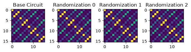
이를 통해 samplex가 예상대로의 샘플을 출력하는지 검증할 수 있습니다. 예를 들어 다음 코드는 바인딩된 회로를 qiskit.quantum_info.Operator 객체로 변환하고 비트 플립 Pauli와 합성하여, 세 무작위화가 모두 기본 회로와 논리적으로 동등한지 시각적으로 확인합니다.

from samplomatic.utils import unbox

# Operator requires that we unpack all of the boxes first
unboxed = unbox(circuit).assign_parameters(inputs["parameter_values"])
# We want to plot unitary matrix amplitudes, so we need to remove the non-unitary measurements
unboxed.remove_final_measurements()
unboxed_unitary = Operator(unboxed)

# Plot magnitudes of the unitary matrix represenation of the circuit
plt.subplot(1, 4, 1)
plt.imshow(np.abs(unboxed_unitary))
plt.title("Base Circuit")

# For each randomization we sampled, plot the unitary matrix representation
for idx in range(3):
    bound_template = template.assign_parameters(outputs["parameter_values"][idx])
    bound_template.remove_final_measurements()

    # The example does measurement twirling by compiling random bitflip gates before the
    # measurements, so we need to undo these at the operator level for each randomization.
    # We do this by casting them to Paulis and composing with the bound circuit's unitary
    alpha_flips = Pauli(([0, 0, 0], outputs["measurement_flips.alpha"][idx, 0]))
    beta_flips = Pauli(([0], outputs["measurement_flips.beta"][idx, 0]))
    flips = beta_flips ^ alpha_flips
    bound_unitary = Operator(bound_template) & flips

    # Plot magnitudes of the unitary matrix represenation of the circuit
    plt.subplot(1, 4, idx + 2)
    plt.imshow(np.abs(bound_unitary))
    plt.title(f"Randomization {idx}")

plt.tight_layout()

마찬가지로 다음 코드는 출력 매개변수 값과 템플릿을 sampler에 전달하여 모든 무작위화에 대해 10,000샷을 시뮬레이션하고, 그 결과의 기댓값(alpha 레지스터에 대해서만)을 기본 회로 시뮬레이션의 기댓값과 비교합니다.

from qiskit.primitives import StatevectorEstimator as Estimator
from qiskit.primitives import StatevectorSampler as Sampler
from qiskit.primitives.containers import BitArray

# simulate some expectation values direction from the base circuit
estimator_job = Estimator().run([(unboxed, ["IZII", "IIZI", "IIIZ"])])
evs = estimator_job.result()[0].data["evs"]

# get the sampler data from each randomization, and do bitflip correction
sampler_job = Sampler().run([(template, outputs["parameter_values"])], shots=10_000)
alpha_data = sampler_job.result()[0].data["alpha"]
alpha_data ^= BitArray.from_bool_array(outputs["measurement_flips.alpha"], "little")

# compare the results
print("  EVs from base circuit:", evs)
print("EVs from randomizations:", alpha_data.expectation_values(["ZII", "IZI", "IIZ"]))

  EVs from base circuit: [0.7819611  0.93553883 0.99500417]
EVs from randomizations: [0.789  0.9366 0.995 ]