QESEM: Qedma의 Qiskit Function

API 참조를 확인하세요

패키지 버전

이 페이지의 코드는 다음 요구 사항을 사용하여 개발되었습니다. 이 버전 이상을 사용하는 것이 좋습니다.

qiskit[all]~=2.5.0
qiskit-ibm-runtime~=0.47.0

참고

Qiskit Functions는 IBM Quantum® Premium Plan, Flex Plan, On-Prem(IBM Quantum Platform API 경유) Plan 사용자에게만 제공되는 실험적 기능입니다. 미리 보기 출시 상태에 있으며 변경될 수 있습니다.

개요

양자 처리 장치는 최근 몇 년간 크게 개선되었지만, 기존 하드웨어의 노이즈와 불완전성으로 인한 오류는 양자 알고리즘 개발자에게 여전히 중심적인 과제입니다. 고전적으로 검증할 수 없는 유틸리티 규모 양자 계산에 가까워짐에 따라, 보장된 정확도로 노이즈를 제거하는 솔루션이 점점 더 중요해지고 있습니다. 이 과제를 극복하기 위해 Qedma는 IBM Quantum Platform에 Qiskit Function으로 원활하게 통합된 양자 오류 완화(QESEM)를 개발했습니다.

QESEM을 사용하면 사용자가 노이즈가 있는 QPU에서 양자 Circuit을 실행하여 근본적인 한계에 가까운 매우 효율적인 QPU 시간 오버헤드로 매우 정확한 오류 없는 결과를 얻을 수 있습니다. 이를 달성하기 위해 QESEM은 오류의 특성화 및 감소를 위해 Qedma가 개발한 독점적 방법 모음을 활용합니다. 오류 감소 기법에는 게이트 최적화, 노이즈 인식 트랜스파일, 오류 억제(ES), 편향 없는 오류 완화(EM)가 포함됩니다. 이 특성화 기반 방법들의 조합으로 사용자는 일반적인 대용량 양자 Circuit에서 신뢰할 수 있고 오류 없는 결과를 얻을 수 있으며, 그렇지 않으면 달성할 수 없는 응용 프로그램을 실현할 수 있습니다.

기본 구성 요소에 대한 전체 설명과 유틸리티 규모 시연은 논문 유틸리티 규모 양자 Circuit을 위한 신뢰할 수 있는 고정확도 오류 완화를 참조하세요.

설명

Qedma의 QESEM 함수를 사용하여 오류 억제 및 완화로 Circuit을 쉽게 추정하고 실행하여 더 큰 Circuit 볼륨과 더 높은 정확도를 달성할 수 있습니다. QESEM을 사용하려면 양자 Circuit, 측정할 Observable 집합, 각 Observable에 대한 목표 통계 정확도, 선택한 QPU를 제공합니다. 목표 정확도로 Circuit을 실행하기 전에 Circuit 실행이 필요 없는 분석적 계산을 기반으로 필요한 QPU 시간을 추정할 수 있습니다. QPU 시간 추정에 만족하면 QESEM으로 Circuit을 실행할 수 있습니다.

Circuit을 실행하면 QESEM은 Circuit에 맞춤화된 장치 특성화 프로토콜을 실행하여 Circuit에서 발생하는 오류에 대한 신뢰할 수 있는 노이즈 모델을 생성합니다. 특성화를 기반으로 QESEM은 먼저 노이즈 인식 트랜스파일을 구현하여 입력 Circuit을 목표 Observable에 영향을 미치는 노이즈를 최소화하는 물리적 Qubit과 게이트 집합으로 매핑합니다. 여기에는 기본적으로 사용 가능한 게이트(IBM® 장치의 CX/CZ)와 QESEM이 최적화한 추가 게이트를 포함하는 QESEM의 확장된 게이트 집합이 포함됩니다. 그런 다음 QESEM은 QPU에서 특성화 기반 ES 및 EM Circuit 집합을 실행하고 측정 결과를 수집합니다. 이 결과들은 고전적으로 후처리되어 요청된 정확도에 해당하는 각 Observable에 대한 편향 없는 기댓값과 오차 막대를 제공합니다.

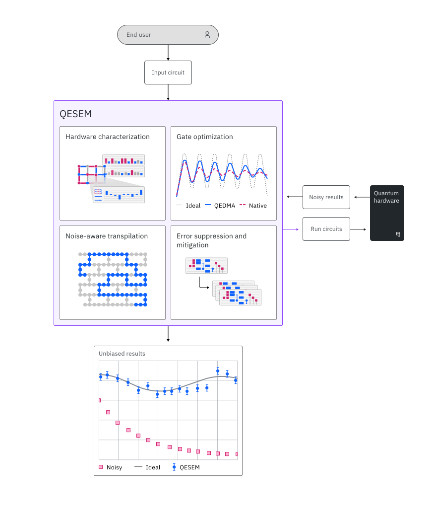QESEM은 다양한 양자 응용 프로그램과 오늘날 달성 가능한 가장 큰 Circuit 볼륨에서 높은 정확도의 결과를 제공하는 것으로 입증되었습니다. QESEM은 아래 벤치마크 섹션에서 시연된 다음과 같은 사용자 지향 기능을 제공합니다:

• 보장된 정확도: QESEM은 Observable의 기댓값에 대한 편향 없는 추정값을 출력합니다. EM 방법은 이론적 보장을 갖추고 있으며, Qedma의 최첨단 특성화와 함께 완화가 사용자 지정 정확도까지 노이즈 없는 Circuit 출력으로 수렴하도록 보장합니다. 체계적인 오류나 편향이 발생하기 쉬운 많은 휴리스틱 EM 방법과 달리, QESEM의 보장된 정확도는 일반적인 양자 Circuit과 Observable에서 신뢰할 수 있는 결과를 보장하는 데 필수적입니다.
• 대규모 QPU로의 확장성: QESEM의 QPU 시간은 Circuit 볼륨에 따라 달라지지만, 그 외에는 qubit 수와 무관합니다. Qedma는 IBM Quantum 127 qubit Eagle 및 133 qubit Heron 장치를 포함하여 오늘날 사용 가능한 가장 큰 양자 장치에서 QESEM을 시연했습니다.
• 응용 프로그램 무관: QESEM은 해밀토니안 시뮬레이션, VQE, QAOA, 진폭 추정을 포함한 다양한 응용 프로그램에서 시연되었습니다. 사용자는 임의의 양자 Circuit과 측정할 Observable을 입력하고 정확한 오류 없는 결과를 얻을 수 있습니다. 유일한 제한은 접근 가능한 Circuit 볼륨과 출력 정확도를 결정하는 하드웨어 사양과 할당된 QPU 시간에 의해 결정됩니다. 대조적으로, 많은 오류 감소 솔루션은 응용 프로그램에 특화되거나 제어되지 않는 휴리스틱을 포함하여 일반적인 양자 Circuit과 응용 프로그램에 적용할 수 없습니다.
• 확장된 게이트 집합: QESEM은 분수 각도 게이트를 지원하고 IBM Quantum Heron 및 Eagle 장치에서 Qedma 최적화 분수 각도 $Rzz(\theta)$ 게이트를 제공합니다. 이 확장된 게이트 집합은 더 효율적인 컴파일을 가능하게 하고 기본 CX/CZ 컴파일에 비해 최대 2배 더 큰 Circuit 볼륨을 실현합니다.
• Multibase Observable: QESEM은 일반 해밀토니안과 같이 많은 비교환 Pauli 문자열로 구성된 입력 Observable을 지원합니다. 측정 기저의 선택과 QPU 리소스 할당(샷 및 Circuit)의 최적화는 요청된 정확도를 위한 필요한 QPU 시간을 최소화하기 위해 QESEM에 의해 자동으로 수행됩니다. 하드웨어 충실도와 실행 속도를 고려하는 이 최적화를 통해 더 깊은 Circuit을 실행하고 더 높은 정확도를 얻을 수 있습니다.

벤치마크

QESEM은 다양한 사용 사례와 응용 프로그램에서 테스트되었습니다. 다음 예제는 QESEM으로 실행할 수 있는 워크로드 유형을 평가하는 데 도움이 됩니다.

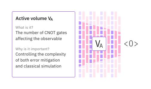
주어진 Circuit과 Observable에 대한 오류 완화와 고전적 시뮬레이션의 어려움을 정량화하는 핵심 지표(성능 지수)는 활성 볼륨입니다: Circuit에서 Observable에 영향을 미치는 CNOT 게이트의 수. 활성 볼륨은 Circuit 깊이와 너비, Observable 가중치, Observable의 라이트콘을 결정하는 Circuit 구조에 따라 달라집니다. 자세한 내용은 2024 IBM Quantum Summit 강연을 참조하세요. QESEM은 고볼륨 레짐에서 특히 큰 가치를 제공하며 일반적인 Circuit과 Observable에 대한 신뢰할 수 있는 결과를 제공합니다.

응용 프로그램	qubit 수	장치	Circuit 설명	정확도	총 시간	런타임 사용
VQE Circuit	8	Eagle (r3)	21개 총 레이어, 9개 측정 기저, 1D 체인	98%	35분	14분
Kicked Ising	28	Eagle (r3)	고유 레이어 3개 x 3단계, 2D heavy-hex 토폴로지	97%	22분	4분
Kicked Ising	28	Eagle (r3)	고유 레이어 3개 x 8단계, 2D heavy-hex 토폴로지	97%	116분	23분
트로터화 해밀토니안 시뮬레이션	40	Eagle (r3)	고유 레이어 2개 x 10 트로터 단계, 1D 체인	97%	3시간	25분
트로터화 해밀토니안 시뮬레이션	119	Eagle (r3)	고유 레이어 3개 x 9 트로터 단계, 2D heavy-hex 토폴로지	95%	6.5시간	45분
Kicked Ising	136	Heron (r2)	고유 레이어 3개 x 15단계, 2D heavy-hex 토폴로지	99%	52분	9분

여기서 정확도는 Observable의 이상적인 값에 대한 상대적인 측정값입니다: $\frac{\langle O \rangle_{ideal} - \epsilon}{\langle O \rangle_{ideal}}$, 여기서 '$\epsilon$'은 완화의 절대 정밀도(사용자 입력으로 설정)이고, $\langle O \rangle_{ideal}$은 노이즈 없는 Circuit에서의 Observable 값입니다. '런타임 사용'은 배치 모드에서의 벤치마크 사용량(개별 Job 사용량의 합계)을 측정하며, '총 시간'은 추가적인 고전 및 통신 시간을 포함하는 세션 모드에서의 사용량(실험 벽시계 시간)을 측정합니다. QESEM은 두 모드 모두에서 실행 가능하므로 사용자는 사용 가능한 리소스를 최대한 활용할 수 있습니다.

28 qubit Kicked Ising Circuit은 ibm_kawasaki의 세 개 연결 루프에서 Shinjo et al.이 연구한 이산 시간 준결정을 시뮬레이션합니다(참조 arXiv 2403.16718 및 Q2B24 Tokyo). 여기서 취한 Circuit 매개변수는 $(\theta_x, \theta_z) = (0.9 \pi, 0)$이며, 강자성 초기 상태 $| \psi_0 \rangle = | 0 \rangle ^{\otimes n}$입니다. 측정된 Observable은 자화의 절댓값 $M = |\frac{1}{28} \sum_{i=0}^{27} \langle Z_i \rangle|$입니다. 유틸리티 규모 Kicked Ising 실험은 ibm_fez의 136개 최고 Qubit에서 실행되었습니다. 이 특정 벤치마크는 Clifford 각도 $(\theta_x, \theta_z) = (\pi, 0)$에서 실행되었으며, 이 각도에서는 활성 볼륨이 Circuit 깊이에 따라 천천히 증가하여 높은 장치 충실도와 함께 짧은 런타임에 높은 정확도를 달성할 수 있습니다.

트로터화 해밀토니안 시뮬레이션 Circuit은 분수 각도의 횡방향 필드 이징 모델에 대한 것입니다: $(\theta_{zz}, \theta_x) = (\pi / 4, \pi /8)$ 및 $(\theta_{zz}, \theta_x) = (\pi / 6, \pi / 8)$(참조 Q2B24 Tokyo). 유틸리티 규모 Circuit은 ibm_brisbane의 119개 최고 Qubit에서 실행되었으며, 40 qubit 실험은 사용 가능한 최고의 체인에서 실행되었습니다. 정확도는 자화에 대해 보고됩니다. 더 높은 가중치의 Observable에 대해서도 높은 정확도의 결과를 얻었습니다.

VQE Circuit은 Deutsches Elektronen-Synchrotron(DESY)의 양자 기술 및 응용 센터 연구자들과 함께 개발되었습니다. 여기서 목표 Observable은 많은 수의 비교환 Pauli 문자열로 구성된 해밀토니안으로, 다중 기저 Observable에 대한 QESEM의 최적화된 성능을 강조합니다. 완화는 고전적으로 최적화된 앤자츠에 적용되었습니다. 이 결과들은 아직 미발표 상태이지만, 유사한 구조적 특성을 가진 다른 Circuit에서도 동일한 품질의 결과를 얻을 수 있습니다.

시작하기

IBM Quantum Platform API 키를 사용하여 인증하고 다음과 같이 QESEM Qiskit Function을 선택하세요. (이 코드 스니펫은 이미 로컬 환경에 계정을 저장했다고 가정합니다.)

# Added by doQumentation — required packages for this notebook
!pip install -q qiskit qiskit-ibm-catalog qiskit-ibm-runtime

import qiskit
from qiskit_ibm_catalog import QiskitFunctionsCatalog

catalog = QiskitFunctionsCatalog(channel="ibm_quantum_platform")

# verify that you have access to the function
catalog.list()

# load the function
qesem_function = catalog.load("qedma/qesem")

예제

시간 추정 작업 예제

시간 추정 작업은 주어진 pub 및 backend_name에 필요한 QPU 시간을 추정하는 데 유용합니다. backend_name은 시뮬레이터 백엔드로도 설정할 수 있습니다. 예를 들어 fake_fez입니다.

QESEM은 준확률적(quasi-probabilistic)이고 특성화 기반의 EM 방법을 사용합니다. 이 방법의 QPU 시간 오버헤드는 대략 다음과 같이 스케일링됩니다.

$T_{QPU} = a \frac{e^{\alpha IF\cdot V_a}}{\epsilon^2} + b$

여기서 $V_a$는 회로의 활성 볼륨, $\epsilon$은 목표 정밀도, $IF$는 네이티브 게이트의 불충실도(infidelity)입니다.

"estimate_time_only": "empirical"은 작업에 필요한 시간을 추정하기 위해 몇 분의 QPU 시간을 사용합니다(백엔드가 실제 장치인 경우; 시뮬레이터인 경우 QPU 시간이 사용되지 않습니다). 이는 일반적으로 약 5분이 걸리지만 10분을 넘지는 않습니다. 경험적 시간 추정 작업과 완화 작업 사이에 불충실도가 크게 변하면 QPU 시간도 크게 변합니다.

시작하려면 주어진 pub에 대해 QESEM을 실행하는 데 필요한 QPU 시간을 추정하는 다음 기본 예제를 시도해 보세요:

# This cell is hidden from users
from qiskit_ibm_runtime import QiskitRuntimeService

service = QiskitRuntimeService()
backend_name = service.least_busy().name

backend_name = "fake_fez"

circ = qiskit.QuantumCircuit(5)
circ.cx(0, 1)
circ.cx(2, 3)
circ.cx(1, 2)
circ.cx(3, 4)

avg_magnetization = qiskit.quantum_info.SparsePauliOp.from_sparse_list(
    [("Z", [q], 1 / 5) for q in range(5)], num_qubits=5
)
other_observable = qiskit.quantum_info.SparsePauliOp.from_sparse_list(
    [("ZZ", [0, 1], 1.0), ("XZ", [1, 4], 0.5)], num_qubits=5
)

time_estimation_job = qesem_function.run(
    pubs=[(circ, [avg_magnetization, other_observable])],
    options={
        "estimate_time_only": "empirical",
    },
    backend_name=backend_name,  # example: "fake_fez", "ibm_fez"
)

time_estimate_result = (
    time_estimation_job.result()
)  # a list of results per pub (circuit)

다음 코드 스니펫은 시간 추정 작업(estimate_time_only가 설정된 경우)에서 다양한 실행 지표를 검색하는 방법을 설명합니다.

pub_result = time_estimate_result[0]

print(
    f"The estimated QPU time for mitigation for this PUB is: {pub_result.metadata['time_estimation_sec']}"
)
print(
    f"The QPU time that this time estimation job took is (here it is 0 because we used fake_fez): {pub_result.metadata['total_qpu_time']}"
)
print(
    f"Gates fidelity measured during the experiment: {pub_result.metadata['gate_fidelities']}"
)
print(f"Total shots: {pub_result.metadata['total_shots']}")
print(f"Resource usage breakdown: {pub_result.metadata['resource_usage']}")

The estimated QPU time for mitigation for this PUB is: 300
The QPU time that this time estimation job took is (here it is 0 because we used fake_fez): 0
Gates fidelity measured during the experiment: {'CZ': 0.9951354916722668, 'ID1Q': 0.9991246627329172}
Total shots: 220000
Resource usage breakdown: {'RUNNING: MAPPING': {'CPU_TIME': 33.6066133165732, 'GPU_TIME': 0.0, 'QPU_TIME': 0.0}, 'RUNNING: OPTIMIZING_FOR_HARDWARE': {'CPU_TIME': 184.53575124032795, 'GPU_TIME': 0.0, 'QPU_TIME': 0.0}, 'RUNNING: WAITING_FOR_QPU': {'CPU_TIME': 0.0, 'GPU_TIME': 0.0, 'QPU_TIME': 0.0}, 'RUNNING: EXECUTING_QPU': {'CPU_TIME': 0.0, 'GPU_TIME': 0.0, 'QPU_TIME': 0.0}, 'RUNNING: POST_PROCESSING': {'CPU_TIME': 0.0, 'GPU_TIME': 0.0, 'QPU_TIME': 0.0}}

경험적 시간 추정이 활성화되면, QESEM은 더 정확한 QPU 시간 추정치를 제공하기 위해 소수의 회로를 실행합니다. 이 회로들의 완화 결과는 작업의 empirical_estimation_mitigation_results 필드에서 확인할 수 있습니다.

이 결과는 제한된 회로 샘플에서 도출된 것이므로, 완전한 QESEM 완화 작업에서 얻은 최종 결과보다 정확도가 현저히 낮습니다. 그러나 회로가 작거나 목표 정밀도가 낮은 경우, 경험적 시간 추정 중에 수행된 완화만으로도 원하는 정밀도에 도달하기에 충분할 수 있으며, 전체 완화 작업이 필요하지 않을 수도 있습니다.

empirical_estimation_mitigation_results 필드는 입력 매개변수별 PrimitiveResult 객체의 리스트입니다. 회로가 매개변수화되지 않은 경우, 이 리스트의 길이는 1이 됩니다.

empirical_estimation_mitigation_results = time_estimate_result[0].metadata[
    "empirical_estimation_mitigation_results"
][0]  # a list per parameter

print("Partial results for the observables:")

print(
    f"    Mitigated expectation values: {empirical_estimation_mitigation_results.data.evs}"
)
print(
    f"    Mitigated error bars: {empirical_estimation_mitigation_results.data.stds}"
)
print(
    f"    Number of shots used for mitigation: {empirical_estimation_mitigation_results.metadata['mitigation_shots']}"
)
transpiled_circ = empirical_estimation_mitigation_results.metadata[
    "transpiled_circ"
]
print(f"    Qubit mapping: {transpiled_circ['qubit_maps']}")
print(
    f"    Number of measurement bases: {transpiled_circ['num_measurement_bases']}\n"
)

# results per obs
emp_obs_results = empirical_estimation_mitigation_results.metadata["results"][
    0
]
# print(f"Results for each observable: {results}")
print("Results for each observable:")

for i, (obs_array, result_dict) in enumerate(emp_obs_results):
    # obs_array, result_dict = results
    print(f"Observable {i+1}: {obs_array}")
    print(
        f"    QESEM mitigated value: {result_dict['qesem']['value']} \u00b1 {result_dict['qesem']['error_bar']}"
    )

Partial results for the observables:
    Mitigated expectation values: [1.00347302 1.00693905]
    Mitigated error bars: [0.00304061 0.00714276]
    Number of shots used for mitigation: 180000
    Qubit mapping: [[[0, 136], [1, 143], [2, 142], [3, 141], [4, 140]]]
    Number of measurement bases: 2

Results for each observable:
Observable 1: ObservablesArray({'IIIIZ': 0.2, 'IIIZI': 0.2, 'IIZII': 0.2, 'IZIII': 0.2, 'ZIIII': 0.2}, shape=())
    QESEM mitigated value: 1.003473015776871 ± 0.0030406128032204015
Observable 2: ObservablesArray({'IIIZZ': 1.0, 'ZIIXI': 0.5}, shape=())
    QESEM mitigated value: 1.0069390542613554 ± 0.0071427606736885925

QESEM 완화 작업 예제

다음 예제는 QESEM Job을 실행합니다:

sample_job = qesem_function.run(
    pubs=[(circ, [avg_magnetization, other_observable])],
    backend_name=backend_name,  # example: "ibm_fez"
    # options = {
    #     "estimate_time_only": "empirical",
    #     "default_precision": 0.2,  # Default precision is applied to all pubs that don't have a precision specified, see API reference for more details
    #     "max_execution_time": 3600,  # You can specify a maximum QPU time in seconds, see API reference for more details
    #     "transpilation_level": "standard",  # "minimal_with_layout_opt" for minimal transpilation, see API reference for more details
    #     "parallel_execution": True,  # True for parallel execution, see API reference for more details
    # },
)

각 입력 필드 및 옵션에 대한 자세한 설명은 QESEM API 참조를 확인하세요. 익숙한 Qiskit Serverless API를 사용하여 Qiskit Function 워크로드의 상태를 확인하거나 결과를 반환할 수 있습니다:

# Print the ID so you can use it later, if necessary
print(sample_job.job_id)
print(sample_job.status())
sample_result = sample_job.result()

3ac6b2df-15b0-4dc0-8f48-cf14bd20a1c8
DONE

다음 코드 스니펫은 완화 결과와 실행 지표를 검색하는 방법을 보여줍니다. 이것들은 QESEM 실행에 다양한 매개변수가 미치는 영향에 대한 더 깊은 이해를 가능하게 하는 필수 데이터를 포함합니다. 연구를 기반으로 논문을 작성할 때도 관련이 있을 수 있습니다.

for pub_idx, pub_result in enumerate(
    sample_result
):  # each element in the list is a result for a different pub, here we sent only one pub
    print(f"\nPUB {pub_idx}:")
    print(
        f"  The QPU time that this job took is (here it is 0 because we used fake_fez): {pub_result.metadata['total_qpu_time']}"
    )
    print(
        f"  Gates fidelity measured during the experiment: {pub_result.metadata['gate_fidelities']}"
    )
    print(f"  Total shots: {pub_result.metadata['total_shots']}")
    print(
        f"  Number of shots used for mitigation: {pub_result.metadata['mitigation_shots']}"
    )
    print(
        f"  Resource usage breakdown: {pub_result.metadata['resource_usage']}"
    )

PUB 0:
  The QPU time that this job took is (here it is 0 because we used fake_fez): 0.0
  Gates fidelity measured during the experiment: {'CZ': 0.9953704216147041, 'ID1Q': 0.9991834123567518}
  Total shots: 446000
  Number of shots used for mitigation: 194000
  Resource usage breakdown: {'RUNNING: MAPPING': {'CPU_TIME': 32.52745003718883, 'GPU_TIME': 0.0, 'QPU_TIME': 0.0}, 'RUNNING: OPTIMIZING_FOR_HARDWARE': {'CPU_TIME': 257.850521848537, 'GPU_TIME': 0.0, 'QPU_TIME': 0.0}, 'RUNNING: WAITING_FOR_QPU': {'CPU_TIME': 0.0, 'GPU_TIME': 0.0, 'QPU_TIME': 0.0}, 'RUNNING: EXECUTING_QPU': {'CPU_TIME': 0.0, 'GPU_TIME': 0.0, 'QPU_TIME': 0.0}, 'RUNNING: POST_PROCESSING': {'CPU_TIME': 0.0, 'GPU_TIME': 0.0, 'QPU_TIME': 0.0}}

metadata["results"]에서 결과는 먼저 회로 인스턴스별로, 그다음 관측량별로 그룹화됩니다.

print("Full QESEM mitigation results:")

for pub_idx, pub_result in enumerate(sample_result):
    print(f"\nPUB {pub_idx}:")

    print(f"  Mitigated expectation values: {pub_result.data.evs}")
    print(f"  Mitigated error bars: {pub_result.data.stds}")
    noisy_results = pub_result.metadata.get("noisy_results")
    print(f"  Unmitigated expectation values: {noisy_results.evs}")
    print(f"  Unmitigated error bars: {noisy_results.stds}")

    print("  Transpiled circuits:")
    for circ_idx, transpiled_circ in enumerate(
        pub_result.metadata["transpiled_circs"]
    ):
        print(f"    Circuit {circ_idx}:")
        # print(f"      Circuit: \n {transpiled_circ['circuit']}") # not printing it because it's long but you can see the transpiled circuit itself
        print(f"      Qubit mapping: {transpiled_circ['qubit_maps']}")
        print(
            f"      Measurement bases: {transpiled_circ['num_measurement_bases']}"
        )

    print("  Results for each observable:")
    for circ_idx, circ_results in enumerate(pub_result.metadata["results"]):
        print(f"    Circuit {circ_idx}:")
        for obs_idx, (obs_array, result_dict) in enumerate(circ_results):
            print(f"      Observable {obs_idx}: {obs_array}")
            print(
                f"        QESEM mitigated value: {result_dict['qesem']['value']} ± {result_dict['qesem']['error_bar']}"
            )
            print(
                f"        Unmitigated value: {result_dict['unmitigated']['value']} ± {result_dict['unmitigated']['error_bar']}"
            )

Full QESEM mitigation results:

PUB 0:
  Mitigated expectation values: [1.00648343 1.00636289]
  Mitigated error bars: [0.00253812 0.00693586]
  Unmitigated expectation values: [0.98031429 0.96357143]
  Unmitigated error bars: [0.00124128 0.00578812]
  Transpiled circuits:
    Circuit 0:
      Qubit mapping: [[[0, 140], [1, 141], [2, 142], [3, 143], [4, 136]]]
      Measurement bases: 2
  Results for each observable:
    Circuit 0:
      Observable 0: ObservablesArray({'IIIIZ': 0.2, 'IIIZI': 0.2, 'IIZII': 0.2, 'IZIII': 0.2, 'ZIIII': 0.2}, shape=())
        QESEM mitigated value: 1.0064834305181962 ± 0.002538119914534849
        Unmitigated value: 0.9803142857142859 ± 0.0012412835813609938
      Observable 1: ObservablesArray({'IIIZZ': 1.0, 'ZIIXI': 0.5}, shape=())
        QESEM mitigated value: 1.0063628870614818 ± 0.006935859820870656
        Unmitigated value: 0.9635714285714285 ± 0.005788121870526659

주요 결과 개요:

• mitigated: 완전히 완화된 QESEM 기댓값입니다.
• unmitigated: 오류 완화가 적용되지 않은 원시 물리적 노이즈 결과입니다.

QESEM 휴리스틱 외삽 결과

단일 precision 부동소수점 값을 사용하는 표준 QESEM 실행에서는 결과에 QESEM 휴리스틱에 사용되는 자동으로 제공되는 노이즈 스케일링 포인트도 포함됩니다. 이러한 포인트는 추가 QPU 리소스 없이 계산됩니다.

스케일 1.0은 판독 완화(REM)가 적용된 물리적 장치 노이즈 수준을 나타내며, 스케일 2.0은 REM이 함께 적용된 보완적인 노이즈 증폭 포인트입니다. 이 포인트들은 qesem_heuristic 결과를 생성하는 데 사용됩니다.

• qesem_heuristic: 사용 가능한 노이즈 스케일 데이터로부터 계산된 ZNE 방식의 추정값입니다. 현재는 지수 외삽법을 사용합니다.

• noise_scaling.results_with_REM: 판독 완화(REM)가 모두 적용된 다양한 노이즈 스케일에서의 기댓값입니다.

미묘하지만 중요한 세부 사항은 스케일 1.0 결과가 unmitigated 결과와 동일하지 않다는 점입니다. 둘 다 물리적 장치 노이즈 수준에 해당하지만, 스케일 1.0 포인트는 판독 완화를 포함하는 반면 unmitigated는 포함하지 않습니다.

print("QESEM heuristic results:")

for pub_idx, pub_result in enumerate(sample_result):
    print(f"\nPUB {pub_idx}:")
    for circ_idx, circ_results in enumerate(pub_result.metadata["results"]):
        print(f"  Circuit {circ_idx}:")
        for obs_idx, (obs_array, result_dict) in enumerate(circ_results):
            print(f"    Observable {obs_idx}: {obs_array}")
            qesem_heuristic = result_dict["qesem_heuristic"][0]
            print("      QESEM heuristic:")
            print(
                f"        Value: {qesem_heuristic['value']} ± {qesem_heuristic['error_bar']}"
            )
            print(
                f"        Extrapolation: {qesem_heuristic['extrapolation']}"
            )
            print(
                f"        Scale factors: {qesem_heuristic['scale_factors']}"
            )
            noise_scaling = result_dict["noise_scaling"]
            print("      Noise scaling results:")
            print(
                f"        Scaling method: {noise_scaling['scaling_method']}"
            )
            print("        Results with Readout mitigation (REM):")
            for rem_result in sorted(
                (
                    item
                    for item in noise_scaling["results_with_REM"]
                    if item["scale"] != 0.0
                ),
                key=lambda item: item["scale"],
            ):
                print(
                    f"          Scale factor {rem_result['scale']}: {rem_result['value']} ± {rem_result['error_bar']}"
                )

QESEM heuristic results:

PUB 0:
  Circuit 0:
    Observable 0: ObservablesArray({'IIIIZ': 0.2, 'IIIZI': 0.2, 'IIZII': 0.2, 'IZIII': 0.2, 'ZIIII': 0.2}, shape=())
      QESEM heuristic:
        Value: 1.0008161638888535 ± 0.0038859458884403964
        Extrapolation: exponential
        Scale factors: [1.0, 2.0]
      Noise scaling results:
        Scaling method: QESEM
        Results with Readout mitigation (REM):
          Scale factor 1.0: 0.9918395459270772 ± 0.0012565417579355634
          Scale factor 2.0: 0.982943441922748 ± 0.0028919278067695018
    Observable 1: ObservablesArray({'IIIZZ': 1.0, 'ZIIXI': 0.5}, shape=())
      QESEM heuristic:
        Value: 0.9960853148925298 ± 0.013811635038961175
        Extrapolation: exponential
        Scale factors: [1.0, 2.0]
      Noise scaling results:
        Scaling method: QESEM
        Results with Readout mitigation (REM):
          Scale factor 1.0: 0.9902860583785115 ± 0.005921236914723409
          Scale factor 2.0: 0.984520565414274 ± 0.006909522262347639

참고

다음 예제들은 기능별 입력과 결과에 초점을 맞추고 있으므로 매번 전체 실행 메트릭을 출력하지는 않습니다. 앞서 표시된 total_qpu_time, gate_fidelities, total_shots, mitigation_shots, resource_usage와 같은 최상위 메타데이터는 이러한 작업에도 사용할 수 있습니다.

백엔드, 관측량, 기본 회로 매개변수를 포함한 이전 예제의 일부 변수는 간결성을 위해 아래에서 재사용됩니다.

참고

다음 예제들은 모두 경험적 시간 추정(empirical time estimation)으로도 실행할 수 있습니다. 이를 활성화하려면 함수 옵션에 "estimate_time_only": "empirical"을 전달하세요.

매개변수화된 회로 예제

많은 알고리즘은 동일한 회로를 여러 매개변수 값에서 평가합니다. 매개변수화된 회로를 하나의 QESEM 작업으로 전송하면 QESEM이 회로 인스턴스 간에 특성화 및 보정을 공유할 수 있어, 개별 작업을 실행하는 것보다 QPU 시간 오버헤드를 줄일 수 있습니다.

매개변수화된 회로를 제출하려면 "minimal_with_layout_opt" 트랜스파일 레벨을 사용해야 합니다. 이 레벨로 제출된 회로는 백엔드에 따라 이미 백엔드의 기본 게이트로 표현되어 있어야 합니다. 이 레벨에서 QESEM은 제출된 구조를 입력 회로와 최대한 가깝게 유지하고, 레이어화(병렬 2-큐비트 게이트 레이어로 연산을 그룹화) 중에 배리어를 준수하며, 고충실도 큐비트 및 장치 연결성에 대한 하드웨어 매핑을 여전히 자동으로 처리합니다.

실제로는 제출 전에 회로를 대상 백엔드의 기본 게이트로 트랜스파일해야 함을 의미합니다. 간단한 기본 게이트 트랜스파일 예제는 아래에 나와 있습니다.

QESEM은 현재 매개변수 집합당 하나의 관측량만 지원합니다. 아래의 두 매개변수 행은 두 개의 관측량과 짝지어집니다. 첫 번째 행은 avg_magnetization으로 측정되고, 두 번째 행은 other_observable로 측정됩니다.

# Transpile to the backend basis gates only. With minimal_with_layout_opt, QESEM handles hardware mapping/connectivity and observable layout internally.
from qiskit_ibm_runtime.fake_provider import FakeFez

backend = FakeFez()
basis = backend.operation_names
print(basis)

param0 = qiskit.circuit.Parameter("param0")
param1 = qiskit.circuit.Parameter("param1")
parametrized_circ = qiskit.QuantumCircuit(5)
parametrized_circ.rx(param0, 0)
parametrized_circ.rx(param1, 1)
parametrized_circ.cx(0, 1)
parametrized_circ.cx(2, 3)
parametrized_circ.cx(1, 2)
parametrized_circ.cx(3, 4)

parametrized_circ = qiskit.transpile(
    parametrized_circ, basis_gates=basis, optimization_level=1
)
parametrized_parameter_values = [[0.5, 0.1], [0.0, 0.6]]
parametrized_observables = [avg_magnetization, other_observable]

parametrized_job = qesem_function.run(
    pubs=[
        (
            parametrized_circ,
            parametrized_observables,
            parametrized_parameter_values,
            0.1,
        )
    ],
    backend_name=backend_name,
    options={
        "max_execution_time": 300,
        "transpilation_level": "minimal_with_layout_opt",
    },
)

print(parametrized_job.job_id)
print(parametrized_job.status())

d1b0e29b-196c-4896-aec6-44a268ebd874
DONE

parametrized_result = parametrized_job.result()

print("Parameterized circuit QESEM results:")

for pub_idx, pub_result in enumerate(parametrized_result):
    print(f"\nPUB {pub_idx}:")
    print(f"  Mitigated expectation values: {pub_result.data.evs}")
    print(f"  Mitigated error bars: {pub_result.data.stds}")
    noisy_results = pub_result.metadata["noisy_results"]
    print(f"  Unmitigated expectation values: {noisy_results.evs}")
    print(f"  Unmitigated error bars: {noisy_results.stds}")
    print("  Results for each parameter value:")
    for param_idx, param_results in enumerate(pub_result.metadata["results"]):
        print(
            f"    Parameter set {param_idx}: {parametrized_parameter_values[param_idx]}"
        )
        for obs_idx, (obs_array, result_dict) in enumerate(param_results):
            print(f"      Observable {obs_idx}: {obs_array}")
            print(
                f"        QESEM mitigated value: {result_dict['qesem']['value']} ± {result_dict['qesem']['error_bar']}"
            )
            print(
                f"        Unmitigated value: {result_dict['unmitigated']['value']} ± {result_dict['unmitigated']['error_bar']}"
            )

Parameterized circuit QESEM results:

PUB 0:
  Mitigated expectation values: [0.92392021 0.82517653]
  Mitigated error bars: [0.00565281 0.00616016]
  Unmitigated expectation values: [0.9028     0.78771429]
  Unmitigated error bars: [0.00335142 0.00925413]
  Results for each parameter value:
    Parameter set 0: [0.5, 0.1]
      Observable 0: ObservablesArray({'IIIIZ': 0.2, 'IIIZI': 0.2, 'IIZII': 0.2, 'IZIII': 0.2, 'ZIIII': 0.2}, shape=())
        QESEM mitigated value: 0.923920210615709 ± 0.005652811570890183
        Unmitigated value: 0.9028 ± 0.0033514176105045447
    Parameter set 1: [0.0, 0.6]
      Observable 0: ObservablesArray({'IIIZZ': 1.0, 'ZIIXI': 0.5}, shape=())
        QESEM mitigated value: 0.8251765289285893 ± 0.006160161743353999
        Unmitigated value: 0.7877142857142858 ± 0.009254130564027902

다중 PUB 예제

다중 PUB 실행은 하나의 QESEM 작업에서 여러 관련 회로를 실행하고자 할 때 유용합니다. 매개변수화된 실행과 마찬가지로, QESEM이 별도의 작업에서 반복하는 대신 회로 인스턴스 간에 특성화 및 보정을 공유할 수 있으므로 오버헤드를 줄일 수 있습니다.

이는 Trotter 유형 워크로드와 같이 공유 레이어 구조를 가진 회로에 특히 유용하며, 이 경우 서로 다른 회로가 동일한 고유 레이어를 재사용합니다. 이러한 경우, 함께 실행하면 독립적인 QESEM 작업에 비해 특성화 비용을 줄일 수 있습니다.

다중 PUB 작업에는 "transpilation_level": "minimal_with_layout_opt"가 필요합니다. 매개변수화된 예제와 마찬가지로, 회로는 제출 전에 대상 백엔드의 기본 게이트로 트랜스파일되어야 합니다. 그러면 QESEM이 장치 연결성, 레이아웃, 고충실도 큐비트로의 매핑을 내부적으로 처리합니다.

아래의 각 PUB에는 하나의 회로와 노트북에서 앞서 사용된 동일한 두 개의 관측량이 포함되어 있으므로, 반환되는 PrimitiveResult에는 입력 회로마다 하나의 PubResult가 포함됩니다.

아래 예제는 동일한 레이어 패턴을 가진 두 개의 간단한 Trotter 회로를 사용합니다. circ_a는 하나의 Trotter 레이어를 가지며, circ_b는 동일한 레이어 패턴을 두 번 반복합니다. 이를 통해 공유 구조가 명시적으로 드러납니다.

def make_trotter_circuit(num_qubits, num_layers, zz_angle=0.2, x_angle=0.1):
    trotter_circ = qiskit.QuantumCircuit(num_qubits)
    for _ in range(num_layers):
        for q in range(num_qubits):
            trotter_circ.rx(x_angle, q)
        trotter_circ.barrier()
        for q in range(0, num_qubits - 1, 2):
            trotter_circ.rzz(zz_angle, q, q + 1)
        trotter_circ.barrier()
        for q in range(1, num_qubits - 1, 2):
            trotter_circ.rzz(zz_angle, q, q + 1)
        trotter_circ.barrier()
    return trotter_circ

circ_a = make_trotter_circuit(num_qubits=5, num_layers=1)
circ_b = make_trotter_circuit(num_qubits=5, num_layers=2)

multi_pubs = [
    (
        qiskit.transpile(qci, basis_gates=basis, optimization_level=1),
        [avg_magnetization, other_observable],
    )
    for qci in [circ_a, circ_b]
]

multi_circ_job = qesem_function.run(
    pubs=multi_pubs,
    backend_name=backend_name,
    options={
        "max_execution_time": 300,
        "transpilation_level": "minimal_with_layout_opt",
        "default_precision": 0.1,
    },
)

print(multi_circ_job.job_id)
print(multi_circ_job.status())

e34565b8-7262-4133-a120-de42ce624a99
DONE

multi_circ_result = multi_circ_job.result()

print("Multi-pub QESEM results:")

for pub_idx, pub_result in enumerate(multi_circ_result):
    print(f"\nPUB {pub_idx}:")
    print(f"  Mitigated expectation values: {pub_result.data.evs}")
    print(f"  Mitigated error bars: {pub_result.data.stds}")
    noisy_results = pub_result.metadata["noisy_results"]
    print(f"  Unmitigated expectation values: {noisy_results.evs}")
    print(f"  Unmitigated error bars: {noisy_results.stds}")
    print("  Results for each observable:")
    for circ_idx, circ_results in enumerate(pub_result.metadata["results"]):
        print(f"    Circuit {circ_idx}:")
        for obs_idx, (obs_array, result_dict) in enumerate(circ_results):
            print(f"      Observable {obs_idx}: {obs_array}")
            print(
                f"        QESEM mitigated value: {result_dict['qesem']['value']} ± {result_dict['qesem']['error_bar']}"
            )
            print(
                f"        Unmitigated value: {result_dict['unmitigated']['value']} ± {result_dict['unmitigated']['error_bar']}"
            )

Multi-pub QESEM results:

PUB 0:
  Mitigated expectation values: [0.99502406 1.02209332]
  Mitigated error bars: [0.00483819 0.00707488]
  Unmitigated expectation values: [0.96934286 0.97271429]
  Unmitigated error bars: [0.00124855 0.00617294]
  Results for each observable:
    Circuit 0:
      Observable 0: ObservablesArray({'IIIIZ': 0.2, 'IIIZI': 0.2, 'IIZII': 0.2, 'IZIII': 0.2, 'ZIIII': 0.2}, shape=())
        QESEM mitigated value: 0.9950240647925642 ± 0.004838188086259301
        Unmitigated value: 0.9693428571428573 ± 0.0012485470362492692
      Observable 1: ObservablesArray({'IIIZZ': 1.0, 'ZIIXI': 0.5}, shape=())
        QESEM mitigated value: 1.0220933230604674 ± 0.007074884384355636
        Unmitigated value: 0.9727142857142859 ± 0.006172939375512439

PUB 1:
  Mitigated expectation values: [0.98850017 1.02555188]
  Mitigated error bars: [0.0077912  0.01672652]
  Unmitigated expectation values: [0.93682857 0.95371429]
  Unmitigated error bars: [0.00156245 0.00665735]
  Results for each observable:
    Circuit 0:
      Observable 0: ObservablesArray({'IIIIZ': 0.2, 'IIIZI': 0.2, 'IIZII': 0.2, 'IZIII': 0.2, 'ZIIII': 0.2}, shape=())
        QESEM mitigated value: 0.988500171577252 ± 0.007791203181151346
        Unmitigated value: 0.9368285714285716 ± 0.001562451883089579
      Observable 1: ObservablesArray({'IIIZZ': 1.0, 'ZIIXI': 0.5}, shape=())
        QESEM mitigated value: 1.02555188098689 ± 0.016726524388086233
        Unmitigated value: 0.9537142857142858 ± 0.006657345655544263

준확률적 오류 튜닝(QET) 예제

준확률적 오류 튜닝(QET)은 선택된 노이즈 스케일 계수에서 기댓값을 요청합니다. 이는 사용자 지정 노이즈 스케일링 연구와 제로 노이즈 외삽 워크플로우에 유용합니다. 스케일 1.0은 물리적 노이즈 수준이며, 0.0과 1.0 사이의 값은 노이즈를 부분적으로 줄이고, 1.0보다 큰 값은 노이즈를 증폭시킵니다.

Qiskit Function과 함께 QET를 사용하려면, PUB precision으로 딕셔너리를 전달하세요. 이 딕셔너리는 요청된 각 noise scale을 해당 목표 precision에 매핑합니다. 반환된 scale-factor 결과는 noise_scaling.results_with_REM에 저장되며 readout mitigation을 포함합니다. 따라서 scale 1.0 지점은 mitigation이 적용되지 않은 값과 동일하지 않은데, 이는 1.0이 readout mitigation을 포함하지만 unmitigated는 그렇지 않기 때문입니다.

스케일이 요청되면 QESEM은 추가 QPU 사용 없이 1.0 주변의 보완적인 스케일도 반환합니다. 예를 들어, 0.5를 요청하면 1.5도 반환될 수 있고, 1.3을 요청하면 0.7도 반환될 수 있습니다. 보완적인 스케일에 대한 precision은 보장되지 않습니다.

noise_scale_precision = {0.5: 0.15, 1.3: 0.2}

qet_job = qesem_function.run(
    pubs=[
        (
            circ,
            [avg_magnetization, other_observable],
            None,
            noise_scale_precision,
        )
    ],
    backend_name=backend_name,
    options={"max_execution_time": 300},
)

print(qet_job.job_id)
print(qet_job.status())

8195fa58-f037-4651-8715-36ce1cdc5521
DONE

qet_result = qet_job.result()

print("QET noise-scaling results:")

for pub_idx, pub_result in enumerate(qet_result):
    print(f"\nPUB {pub_idx}:")
    noisy_results = pub_result.metadata["noisy_results"]
    print(f"  Unmitigated expectation values: {noisy_results.evs}")
    print(f"  Unmitigated error bars: {noisy_results.stds}")
    print("  Results for each observable:")
    for circ_idx, circ_results in enumerate(pub_result.metadata["results"]):
        print(f"    Circuit {circ_idx}:")
        for obs_idx, (obs_array, result_dict) in enumerate(circ_results):
            print(f"      Observable {obs_idx}: {obs_array}")
            noise_scaling = result_dict["noise_scaling"]
            print(
                f"        Scaling method: {noise_scaling['scaling_method']}"
            )
            print("        Results with Readout mitigation (REM):")
            for rem_result in sorted(
                (
                    item
                    for item in noise_scaling["results_with_REM"]
                    if item["scale"] != 0.0
                ),
                key=lambda item: item["scale"],
            ):
                print(
                    f"          Scale factor {rem_result['scale']}: {rem_result['value']} ± {rem_result['error_bar']}"
                )

QET noise-scaling results:

PUB 0:
  Unmitigated expectation values: [0.97822857 0.96171429]
  Unmitigated error bars: [0.00123812 0.00672958]
  Results for each observable:
    Circuit 0:
      Observable 0: ObservablesArray({'IIIIZ': 0.2, 'IIIZI': 0.2, 'IIZII': 0.2, 'IZIII': 0.2, 'ZIIII': 0.2}, shape=())
        Scaling method: QESEM
        Results with Readout mitigation (REM):
          Scale factor 0.5: 0.9938730340199383 ± 0.0032116907357568275
          Scale factor 0.7: 0.9963976191853445 ± 0.00036300258869586616
          Scale factor 1.0: 0.9898115079506586 ± 0.0012525947426560995
          Scale factor 1.3: 0.9864667065580341 ± 0.002633221613518526
          Scale factor 1.5: 0.9838755527197551 ± 0.002948417797996015
      Observable 1: ObservablesArray({'IIIZZ': 1.0, 'ZIIXI': 0.5}, shape=())
        Scaling method: QESEM
        Results with Readout mitigation (REM):
          Scale factor 0.5: 1.0006538544450332 ± 0.002121742014777343
          Scale factor 0.7: 1.0004159801523036 ± 0.0021671375357823794
          Scale factor 1.0: 0.9898058846339917 ± 0.00690183710903159
          Scale factor 1.3: 0.9948946719997267 ± 0.002146532859610311
          Scale factor 1.5: 0.9927220368192772 ± 0.0020875057190323882

오류 메시지 가져오기

워크로드 상태가 ERROR인 경우, job.result()를 사용하여 오류 메시지를 다음과 같이 가져오세요:

# Get the result and truncate for readability
result = sample_job.result()
result_str = str(result)
max_length = 500  # Adjust this value as necessary

if len(result_str) > max_length:
    truncated = (
        result_str[:max_length]
        + f"... (truncated {len(result_str) - max_length} characters)"
    )
else:
    truncated = result_str

print(truncated)

PrimitiveResult([PubResult(data=DataBin(evs=np.ndarray(<shape=(2,), dtype=float64>), stds=np.ndarray(<shape=(2,), dtype=float64>), shape=(2,)), metadata={'gate_fidelities': {'CZ': 0.9979444718552628, 'ID1Q': 0.9991994239814883}, 'total_shots': 498600, 'mitigation_shots': 223400, 'transpiled_circs': [{'circuit': 'OPENQASM 3.0;\ninclude "stdgates.inc";\nbit[76] c0;\nqubit[76] q0;\nrx(0) q0[54];\nrx(0) q0[59];\nrx(0) q0[75];\nrz(pi/2) q0[54];\nrz(pi/2) q0[59];\nrz(pi/2) q0[75];\nrx(pi/2) q0[54];\nr... (truncated 3771 characters)

지원 받기

Qedma 지원팀이 도움을 줍니다! QESEM Qiskit Function을 사용하면서 문제가 발생하거나 질문이 있으시면 주저하지 마시고 연락하세요. 저희의 지식이 풍부하고 친절한 지원 직원이 기술적 우려나 문의 사항을 도와드릴 준비가 되어 있습니다.

도움을 받으시려면 support@qedma.com으로 이메일을 보내세요. 신속하고 정확한 답변을 제공할 수 있도록 경험하고 있는 문제에 대한 가능한 한 많은 세부 사항을 포함해 주세요. 전용 Qedma POC 담당자에게 이메일이나 전화로 연락할 수도 있습니다.

더 효율적으로 도움을 드리기 위해 연락하실 때 다음 정보를 제공해 주세요:

• 문제에 대한 상세한 설명

• Job ID

• 관련 오류 메시지 또는 코드

저희 Qiskit Function을 통해 최고의 경험을 드릴 수 있도록 신속하고 효과적인 지원을 제공하려고 노력하고 있습니다.

저희는 항상 제품을 개선하고 여러분의 제안을 환영합니다! 서비스를 향상시키거나 원하는 기능에 대한 아이디어가 있으시면 support@qedma.com으로 의견을 보내주세요.

다음 단계

권장 사항

• Qedma QESEM 접근 요청.

• 이 Qiskit Function의 API 참조를 방문하세요.

• QESEM 함수를 사용하여 2D 기울어진 필드 이징 시뮬레이션하기 튜토리얼을 시도해 보세요.

• Aharonov, D., et al. (2025). Reliable high-accuracy error mitigation for utility-scale quantum circuits. arXiv preprint arXiv:2508.10997를 검토하세요.

• Aharonov, D., et al. (2025). Syndrome aware mitigation of logical errors. arXiv preprint arXiv:2508.10997를 검토하세요.

• Aharonov, D., et al. (2025). On the Importance of Error Mitigation for Quantum Computation. arXiv preprint arXiv:2512.23810를 검토하세요.

• Bauman, N. P., et al. (2025). Coupled Cluster Downfolding Theory in Simulations of Chemical Systems on Quantum Hardware. arXiv preprint arXiv:2507.01199를 검토하세요.

• Goldack, M., et al. (2026). Computing Statistical Properties of Velocity Fields on Current Quantum Hardware. arXiv preprint arXiv:2601.10166를 검토하세요.

• Sakuma, R., et al. (2026). Point-group symmetry analysis of many-electron wavefunctions on a quantum computer arXiv preprint arXiv:2605.24824를 검토하세요.