Performance Management: Q-CTRL Fire Opal의 Qiskit Function

API 참조를 참조하세요

참고

Qiskit Functions는 IBM Quantum® Premium Plan, Flex Plan, On-Prem(IBM Quantum Platform API 경유) Plan 사용자에게만 제공되는 실험적 기능입니다. 현재 미리보기 릴리스 상태이며 변경될 수 있습니다.

Package versions

이 페이지의 코드는 다음 요구 사항을 사용하여 개발되었습니다. 이러한 버전 이상을 사용하는 것을 권장합니다.

qiskit[all]~=2.3.1
qiskit-ibm-runtime~=0.45.1

개요

Fire Opal Performance Management를 사용하면 양자 하드웨어 전문가가 아니더라도 누구나 대규모 양자 컴퓨터에서 의미 있는 결과를 쉽게 얻을 수 있습니다. Fire Opal Performance Management로 Circuit을 실행하면 AI 기반 오류 억제 기술이 자동으로 적용되어, 더 많은 Gate와 Qubit을 사용하는 더 큰 문제로 확장할 수 있습니다. 이 방식은 추가 오버헤드 없이 정확한 답을 얻는 데 필요한 샷 수를 줄여주어, 컴퓨팅 시간과 비용을 크게 절감할 수 있습니다.

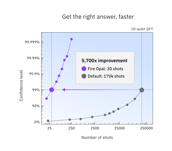
Performance Management는 오류를 억제하여 잡음이 많은 하드웨어에서 정확한 답을 얻을 확률을 높여줍니다. 즉, 신호 대 잡음비를 향상시킵니다. 아래 이미지는 Performance Management로 향상된 정확도가 10-Qubit 양자 푸리에 변환(Quantum Fourier Transform) 알고리즘에서 추가 샷의 필요성을 어떻게 줄이는지 보여줍니다. Q-CTRL은 단 30샷으로 99% 신뢰 임계값에 도달하는 반면, 기본값(QiskitRuntime Sampler, optimization_level=3, resilience_level=1, ibm_sherbrooke)은 170,000샷이 필요합니다. 더 빠르게 정확한 답을 얻음으로써 상당한 컴퓨팅 런타임을 절약할 수 있습니다.

Performance Management 함수는 모든 알고리즘에 사용할 수 있으며, 표준 IBM Quantum 프리미티브 대신 쉽게 사용할 수 있습니다. 내부적으로 여러 오류 억제 기술이 함께 작동하여 런타임에 오류가 발생하는 것을 방지합니다. 모든 Fire Opal 파이프라인 메서드는 사전 구성되어 있으며 알고리즘에 구애받지 않으므로, 별도의 설정 없이 항상 최상의 성능을 발휘합니다.

Performance Management에 대한 액세스 권한을 얻으려면 Q-CTRL에 문의하세요.

설명

Fire Opal Performance Management는 IBM Quantum 프리미티브와 유사한 두 가지 실행 옵션을 제공하므로, Q-CTRL Sampler와 Estimator로 손쉽게 교체하여 사용할 수 있습니다. Performance Management 함수 사용의 일반적인 워크플로는 다음과 같습니다:

1. Circuit을 정의합니다(Estimator의 경우 연산자도 함께 정의).
2. Circuit을 실행합니다.
3. 결과를 조회합니다.

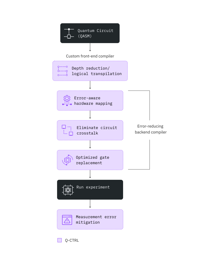
하드웨어 잡음을 줄이기 위해 Fire Opal은 다음 이미지에 나타난 다양한 AI 기반 오류 억제 기술을 활용합니다. Fire Opal을 사용하면 전체 파이프라인이 완전히 자동화되어 별도의 구성이 필요 없습니다.

Fire Opal의 파이프라인은 양자 런타임 증가나 추가 물리 Qubit과 같은 오버헤드의 필요성을 없애줍니다. 단, 클래식 처리 시간은 여전히 고려해야 합니다(벤치마크 섹션에서 추정치를 참고하세요. "총 시간"은 클래식 및 양자 처리 시간 모두를 반영합니다). 샘플링 형태의 오버헤드가 필요한 오류 완화(error mitigation)와 달리, Fire Opal의 오류 억제는 Gate 및 펄스 수준 모두에서 작동하여 다양한 잡음 원인을 해결하고 오류 발생 가능성을 방지합니다. 오류를 사전에 방지함으로써 비용이 큰 사후 처리의 필요성을 없애줍니다.

아래 이미지는 Fire Opal Performance Management가 자동화하는 오류 억제 방법을 보여줍니다.

이 함수는 Sampler와 Estimator 두 가지 프리미티브를 제공하며, 두 프리미티브의 입력 및 출력은 모두 IBM Quantum V2 프리미티브의 구현 사양을 확장합니다.

벤치마크

발표된 알고리즘 벤치마킹 결과는 Bernstein-Vazirani, 양자 푸리에 변환(Quantum Fourier Transform), Grover 탐색, 양자 근사 최적화 알고리즘(QAOA), 변분 양자 고유값 계산(VQE) 등 다양한 알고리즘에서 성능이 크게 향상되었음을 보여줍니다. 이 섹션의 나머지 부분에서는 실행 가능한 알고리즘 유형과 예상 성능 및 런타임에 대한 자세한 정보를 제공합니다.

다음의 독립적인 연구들은 Q-CTRL의 Performance Management가 기록적인 규모의 알고리즘 연구를 가능하게 한다는 것을 보여줍니다:

• Parametrized Energy-Efficient Quantum Kernels for Network Service Fault Diagnosis - 최대 50-Qubit 양자 커널 학습
• Tensor-based quantum phase difference estimation for large-scale demonstration - 최대 33-Qubit 양자 위상 추정
• Hierarchical Learning for Quantum ML: Novel Training Technique for Large-Scale Variational Quantum Circuits - 최대 21-Qubit 양자 데이터 로딩

다음 표는 ibm_fez에서 수행된 이전 벤치마킹 실행의 정확도 및 런타임에 대한 대략적인 가이드를 제공합니다. 다른 디바이스에서의 성능은 다를 수 있습니다. 사용 시간은 Circuit당 10,000샷을 기준으로 합니다. "Qubit 수"는 엄격한 제한이 아니라 극도로 일관된 솔루션 정확도를 기대할 수 있는 대략적인 임계값을 나타냅니다. 더 큰 문제 규모도 성공적으로 해결된 바 있으며, 이러한 한계를 넘어 테스트해 보는 것을 권장합니다.

예시	qubit 수	정확도	정확도 측정 기준	총 시간(초)	런타임 사용량(초)	Primitive (모드)
Bernstein–Vazirani	50Q	100%	성공률(정확한 답이 가장 높은 카운트 비트스트링인 실행 비율)	10	8	Sampler
양자 푸리에 변환(Quantum Fourier Transform)	30Q	100%	성공률(정확한 답이 가장 높은 카운트 비트스트링인 실행 비율)	10	8	Sampler
양자 위상 추정(Quantum Phase Estimation)	30Q	99.9998%	발견된 각도의 정확도: 1- abs(real_angle - angle_found)/pi	10	8	Sampler
양자 시뮬레이션: 이징 모델(15단계)	20Q	99.775%	$A$(아래 정의 참고)	60(단계당)	15(단계당)	Estimator
양자 시뮬레이션 2: 분자 동역학(20개 시간 포인트)	34Q	96.78%	$A_{mean}$(아래 정의 참고)	10(시간 포인트당)	6(시간 포인트당)	Estimator

기댓값 측정의 정확도 정의 - 측정 기준 $A$는 다음과 같이 정의됩니다:

$$A = 1 - \frac{|\epsilon^{ideal} - \epsilon^{meas}|}{\epsilon^{ideal}_{max} - \epsilon^{ideal}_{min}},$$

여기서 $\epsilon^{ideal}$ = 이상적인 기댓값, $\epsilon^{meas}$ = 측정된 기댓값, $\epsilon^{ideal}_{max}$ = 이상적인 최대값, $\epsilon^{ideal}_{min}$ = 이상적인 최소값입니다. $A_{mean}$은 여러 측정에 걸친 $A$ 값의 평균입니다.

이 측정 기준은 달성 가능한 값의 범위에서 전역적 이동 및 스케일링에 불변이기 때문에 사용됩니다. 즉, 가능한 기댓값의 범위를 높이거나 낮추거나 분산을 늘리더라도 $A$의 값은 일관되게 유지됩니다.

시작하기

Fire Opal Performance Management는 권장 버전인 Qiskit v2.0.0을 사용합니다. 지원되는 버전은 Qiskit >=v2.0.0입니다. IBM Quantum Platform API 키를 사용하여 인증하고, 다음과 같이 Qiskit Function을 선택합니다. (이 코드 조각은 이미 로컬 환경에 계정을 저장했다고 가정합니다.)

# Added by doQumentation — required packages for this notebook
!pip install -q matplotlib numpy qiskit qiskit-ibm-catalog qiskit-ibm-runtime

# This cell is hidden from users. It hides the "...You have imported samplomatic..." warning.
import warnings

warnings.filterwarnings("ignore", message=".*You have imported samplomatic*")

from qiskit_ibm_catalog import QiskitFunctionsCatalog

catalog = QiskitFunctionsCatalog(channel="ibm_quantum_platform")

# verify that you have access to the function
catalog.list()

[QiskitFunction(qunova/hivqe-chemistry),
 QiskitFunction(global-data-quantum/quantum-portfolio-optimizer),
 QiskitFunction(algorithmiq/tem),
 QiskitFunction(qedma/qesem),
 QiskitFunction(multiverse/singularity),
 QiskitFunction(ibm/circuit-function),
 QiskitFunction(q-ctrl/optimization-solver),
 QiskitFunction(colibritd/quick-pde),
 QiskitFunction(q-ctrl/performance-management),
 QiskitFunction(kipu-quantum/iskay-quantum-optimizer)]

# Access Function
perf_mgmt = catalog.load("q-ctrl/performance-management")

이 함수가 모든 IBM 백엔드를 지원하나요?

이 함수가 현재 지원하지 않는 백엔드를 사용하려면, Q-CTRL에 문의하여 지원을 추가하세요.

Estimator 프리미티브

Estimator 예시

Fire Opal Performance Management의 Estimator 프리미티브를 사용하여 단일 Circuit-관측량 쌍의 기댓값을 구합니다. qiskit-ibm-catalog 및 qiskit 패키지 외에도, 이 예시를 실행하려면 numpy 패키지도 필요합니다. IPython 커널을 사용하는 노트북에서 이 예시를 실행하는 경우, 다음 셀의 주석을 해제하여 패키지를 설치할 수 있습니다.

# %pip install numpy

1. Circuit 생성

예시로, Performance Management 함수에 입력할 무작위 에르미트 연산자와 관측량을 생성합니다.

import numpy as np
from qiskit.circuit.library import iqp
from qiskit.quantum_info import random_hermitian, SparsePauliOp

n_qubits = 50

# Generate a random circuit
mat = np.real(random_hermitian(n_qubits, seed=1234))
circuit = iqp(mat)
circuit.measure_all()

# Define observables as a string
observable = SparsePauliOp("Z" * n_qubits)

# Create PUB tuple
estimator_pubs = [(circuit, observable)]

2. Circuit 실행

Circuit을 실행하고, 선택적으로 Backend와 샷 수를 정의합니다.

# This cell is hidden from users
from qiskit_ibm_runtime import QiskitRuntimeService

service = QiskitRuntimeService()
backend_name = service.least_busy().name

# Run the circuit using Estimator
qctrl_estimator_job = perf_mgmt.run(
    primitive="estimator",
    pubs=estimator_pubs,
    backend_name=backend_name,
)

익숙한 Qiskit Serverless API를 사용하여 Qiskit Function 워크로드의 상태를 확인할 수 있습니다:

qctrl_estimator_job.status()

'QUEUED'

3. 결과 조회

# Retrieve the counts from the result list
result = qctrl_estimator_job.result()

결과는 Estimator 결과와 동일한 형식을 가집니다:

import numpy

result_str = str(result)

with numpy.printoptions(threshold=200):
    print(
        f"The result of the submitted job had {len(result)} PUB "
        f"and has a value:\n {result[0]}\n"
    )

print("The associated PubResult of this job has the following DataBins:")
print(f"{result[0].data}\n")

print(f"And this DataBin has attributes: {result[0].data.keys()}")

print("The expectation values measured from this PUB are:")
print(f"{result[0].data.evs}")

The result of the submitted job had 1 PUB
The result of the submitted job had 1 PUB and has a value:
 PubResult(data=DataBin(evs=0.0195, stds=0.9998098569228051), metadata={'precision': None})

The associated PubResult of this job has the following DataBins:
DataBin(evs=0.0195, stds=0.9998098569228051)

And this DataBin has attributes: dict_keys(['evs', 'stds'])
The expectation values measured from this PUB are:
0.0195

Sampler 프리미티브

Sampler 예제

Fire Opal Performance Management의 Sampler 프리미티브를 사용하여 Bernstein–Vazirani Circuit을 실행합니다. 이 알고리즘은 블랙박스 함수의 출력으로부터 숨겨진 문자열을 찾는 데 사용되며, 정답이 하나뿐이기 때문에 일반적인 벤치마킹 알고리즘으로 활용됩니다. 1. Circuit 생성

알고리즘의 정답인 숨겨진 비트스트링과 Bernstein–Vazirani Circuit을 정의합니다. circuit_width를 변경하는 것만으로 Circuit의 너비를 조정할 수 있습니다.

import qiskit

circuit_width = 35
hidden_bitstring = "1" * circuit_width

# Create circuit, reserving one qubit for BV oracle
bv_circuit = qiskit.QuantumCircuit(circuit_width + 1, circuit_width)
bv_circuit.x(circuit_width)
bv_circuit.h(range(circuit_width + 1))
for input_qubit, bit in enumerate(reversed(hidden_bitstring)):
    if bit == "1":
        bv_circuit.cx(input_qubit, circuit_width)
bv_circuit.barrier()
bv_circuit.h(range(circuit_width + 1))
bv_circuit.barrier()
for input_qubit in range(circuit_width):
    bv_circuit.measure(input_qubit, input_qubit)

# Create PUB tuple
sampler_pubs = [(bv_circuit,)]

2. Circuit 실행

Circuit을 실행하고, 선택적으로 Backend와 샷 수를 정의합니다.

# Run the circuit using Sampler
qctrl_sampler_job = perf_mgmt.run(
    primitive="sampler",
    pubs=sampler_pubs,
    backend_name=backend_name,
)

다음과 같이 Qiskit Function 워크로드의 상태를 확인하거나 결과를 반환할 수 있습니다.

# Print the ID so you can use it later, if necessary
print(qctrl_sampler_job.job_id)

qctrl_sampler_job.status()

60fe2fa1-a860-43e4-8615-c6ac4180f93b

'QUEUED'

3. 결과 조회

# Retrieve the job results
sampler_result = qctrl_sampler_job.result()

# Get results for the first (and only) PUB
pub_result = sampler_result[0]
counts = pub_result.data.c.get_counts()

print("Counts for the meas output register (limited to 30 results):")
for i, (bitstring, count) in enumerate(counts.items()):
    if i >= 50:
        print(f"  ... ({len(counts) - 30} more items)")
        break
    print(f"  {bitstring}: {count}")

Counts for the meas output register (limited to 30 results):
  11111111111111111111111111111111111: 1661
  11111111111111111111111111110111111: 60
  11111111111111111111111111111101111: 54
  11111111111111111111111111111110111: 54
  11111111111111011111111111111111111: 46
  11111111111111111110111111111111111: 44
  11111111111111111111111101111111111: 42
  11111111111111111111111110111111111: 42
  11111111111111110111111111111111111: 41
  11111111111111111111111111111111101: 39
  11111111111111111111101111111111111: 38
  11111111111111111111110111111111111: 38
  11111111111111111111111111101111111: 37
  11111111111111111111111111111111110: 36
  11111111111110111111111111111111111: 35
  11111111111111111111111111111011111: 32
  11111111111111101111111111111111111: 32
  01111111111111111111111111111111111: 27
  11111111111111111011111111111111111: 23
  11111111101111111111111111111111111: 22
  11111111111111111111111111111111011: 21
  11111111011111111111111111111111111: 20
  00000000000000011111111111111111111: 18
  11111111111111111111110101111111111: 18
  00000001111111111111111111111111111: 17
  11111111001111111111111111111111111: 16
  11101111111111111111111111111111111: 16
  11111111111101111111111111111111111: 16
  00000101111111111111111111111111111: 13
  11111111111111111111111011111111111: 13
  11111111111111111111111110101111111: 13
  11111111111111111101111111111111111: 12
  10111111111111111111111111111111111: 12
  11111111111111111111111110001111111: 12
  00000000000000000011111111111111111: 11
  11111111111111111111111111111110110: 10
  00000000000000000000000001111111111: 10
  11111111111011111111111111111111111: 9
  11111111111111101011111111111111111: 9
  00000000011111111111111111111111111: 8
  10101111111111111111111111111111111: 8
  00000000000000000000000001011111111: 8
  11111111111111111111111111111111001: 8
  00000111111111111111111111111111111: 7
  11111111111111111111111111111101110: 7
  11111111110111111111111111111111111: 7
  00000000000001011111111111111111111: 6
  00000000000000001111111111111111111: 6
  00000000000000000001011111111111111: 6
  11111111111111111111111111011111111: 6
  ... (1050 more items)

3. 상위 비트스트링 플로팅

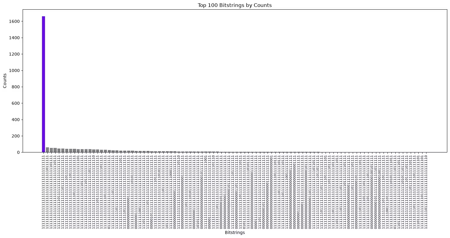
가장 높은 카운트를 가진 비트스트링을 플로팅하여 숨겨진 비트스트링이 최빈값이었는지 확인하세요.

import matplotlib.pyplot as plt

def plot_top_bitstrings(counts_dict, hidden_bitstring=None):
    # Sort and take the top 100 bitstrings
    top_100 = sorted(counts_dict.items(), key=lambda x: x[1], reverse=True)[
        :100
    ]
    if not top_100:
        print("No bitstrings found in the input dictionary.")
        return

    # Unzip the bitstrings and their counts
    bitstrings, counts = zip(*top_100)

    # Assign colors: purple if the bitstring matches hidden_bitstring,
    # otherwise gray
    colors = [
        "#680CE9" if bit == hidden_bitstring else "gray" for bit in bitstrings
    ]

    # Create the bar plot
    plt.figure(figsize=(15, 8))
    plt.bar(
        range(len(bitstrings)), counts, tick_label=bitstrings, color=colors
    )

    # Rotate the bitstrings for better readability
    plt.xticks(rotation=90, fontsize=8)
    plt.xlabel("Bitstrings")
    plt.ylabel("Counts")
    plt.title("Top 100 Bitstrings by Counts")

    # Show the plot
    plt.tight_layout()
    plt.show()

숨겨진 비트스트링은 보라색으로 강조 표시되며, 카운트가 가장 높은 비트스트링이어야 합니다.

plot_top_bitstrings(counts, hidden_bitstring)

Changelog

• 2026-02-20: 지원 중단 공지 - provider_job_ids 메타데이터 필드는 버전 0.13.0에서 30일 후 지원이 중단될 예정입니다. 사용자는 런타임 서비스의 job_id() 메서드를 통해 작업 ID에 액세스할 수 있습니다.

• 2026-02-11: ibm_miami에 대한 지원이 추가되었으며, PubResult에 실행 메타데이터가 추가되었습니다.

지원 받기

질문이나 문제가 있으시면 Q-CTRL에 문의하세요.

다음 단계

권장 사항

• Q-CTRL Performance Management 접근 권한을 신청하세요.

• 이 Qiskit Function의 API 참조를 방문하세요.

• Q-CTRL Performance Management를 사용한 횡방향 장 이징 모델 튜토리얼을 시도해 보세요.

• Q-CTRL Qiskit Functions를 사용한 양자 위상 추정 튜토리얼을 시도해 보세요.

• Mundada P. S., et al. (2023). Experimental Benchmarking of an Automated Deterministic Error-Suppression Workflow for Quantum Algorithms. Physical Review Applied, 20, 2를 검토하세요.

• Kanno, S., et al. (2025). Tensor-based quantum phase difference estimation for large-scale demonstration. arXiv preprint arXiv:2408.04946를 검토하세요.

• SoftBank Corp, Demonstration Experiment of a Communication Service Fault Diagnosis System Using Quantum Machine Learning (blog), 30 August, 2024를 검토하세요.

• Yamauchi, H., et al. (2024). Parametrized Energy-Efficient Quantum Kernels for Network Service Fault Diagnosis. arXiv preprint arXiv:2405.09724v1를 검토하세요.

• Yamauchi, H., et al. (2025). Quantum spectroscopy of topological dynamics via a supersymmetric Hamiltonian. arXiv preprint arXiv:2511.23169v1를 검토하세요.

• Wang, Y., et al. (2025). Δ-Motif: Subgraph Isomorphism at Scale via Data-Centric Parallelism. arXiv preprint arXiv:2508.21287를 검토하세요.

• Paterakis, N. G., et al. (2025). Quantum Computing in the Computational Landscape of Power Electronics: Vision and Reality. arXiv preprint arXiv:2507.02577를 검토하세요.

• Gharibyan, H., et al. (2023). Hierarchical Learning for Quantum ML: Novel Training Technique for Large-Scale Variational Quantum Circuits. arXiv preprint arXiv:2311.12929를 검토하세요.

• Mitsubishi Chemical Corp 사례 연구를 검토하세요.

• Redacted bank 사례 연구를 검토하세요.

• BlueQubit 사례 연구를 검토하세요.