Q-CTRL 성능 관리를 활용한 횡자기장 이징 모델

사용량 추정치: Heron r2 프로세서에서 약 2분. (참고: 이는 추정치이며, 실제 실행 시간은 다를 수 있습니다.)

배경

횡자기장 이징 모델(TFIM)은 양자 자성 및 상전이 연구에서 중요한 모델입니다. 이 모델은 격자 위에 배열된 스핀 집합을 기술하며, 각 스핀은 이웃 스핀과 상호작용하는 동시에 양자 요동을 유발하는 외부 자기장의 영향을 받습니다.

이 모델을 시뮬레이션하는 일반적인 방법은 Trotter 분해를 사용하여 시간 진화 연산자를 근사하는 것입니다. 이를 통해 단일 Qubit 회전과 얽힘 두 Qubit 상호작용을 교대로 적용하는 Circuit을 구성합니다. 그러나 실제 하드웨어에서의 시뮬레이션은 노이즈와 디코히어런스로 인해 어려우며, 이로 인해 실제 동역학과의 편차가 발생합니다. 이를 극복하기 위해 Qiskit Function으로 제공되는 Q-CTRL의 Fire Opal 오류 억제 및 성능 관리 도구를 사용합니다(Fire Opal 문서 참조). Fire Opal은 동적 디커플링, 고급 레이아웃, 라우팅 및 기타 오류 억제 기법을 자동으로 적용하여 Circuit 실행을 최적화하며, 모두 노이즈 감소를 목표로 합니다. 이러한 개선을 통해 하드웨어 결과가 무노이즈 시뮬레이션과 더 가깝게 일치하므로, 더 높은 충실도로 TFIM 자화 동역학을 연구할 수 있습니다.

이 튜토리얼에서는 다음을 수행합니다:

• 연결된 스핀 삼각형 그래프 위에 TFIM 해밀토니안 구성
• 다양한 깊이의 Trotter 회로를 사용한 시간 진화 시뮬레이션
• 시간에 따른 단일 Qubit 자화 $\langle Z_i \rangle$ 계산 및 시각화
• 기본 시뮬레이션과 Q-CTRL Fire Opal 성능 관리를 사용한 하드웨어 실행 결과 비교

개요

횡자기장 이징 모델(TFIM)은 양자 상전이의 핵심 특성을 포착하는 양자 스핀 모델입니다. 해밀토니안은 다음과 같이 정의됩니다:

$$H = -J \sum_{i} Z_i Z_{i+1} - h \sum_{i} X_i$$

여기서 $Z_i$와 $X_i$는 Qubit $i$에 작용하는 파울리 연산자이고, $J$는 이웃 스핀 사이의 결합 강도이며, $h$는 횡자기장의 강도입니다. 첫 번째 항은 고전적인 강자성 상호작용을 나타내며, 두 번째 항은 횡자기장을 통해 양자 요동을 도입합니다. TFIM 동역학을 시뮬레이션하기 위해 연결된 스핀 삼각형의 사용자 정의 그래프를 기반으로 RX 및 RZZ Gate 레이어를 통해 구현된 단일 시간 진화 연산자 $e^{-iHt}$의 Trotter 분해를 사용합니다. 시뮬레이션은 Trotter 단계가 증가함에 따라 자화 $\langle Z \rangle$이 어떻게 변화하는지 탐구합니다.

제안된 TFIM 구현의 성능은 무노이즈 시뮬레이션과 노이즈 있는 Backend를 비교하여 평가됩니다. Fire Opal의 향상된 실행 및 오류 억제 기능을 사용하여 실제 하드웨어의 노이즈 영향을 완화하고, $\langle Z_i \rangle$ 및 상관관계 $\langle Z_i Z_j \rangle$와 같은 스핀 관측값에 대해 더 신뢰할 수 있는 추정치를 얻습니다.

요구 사항

이 튜토리얼을 시작하기 전에 다음이 설치되어 있는지 확인하세요:

• Qiskit SDK v1.4 이상 (시각화 지원 포함)
• Qiskit Runtime v0.40 이상 (pip install qiskit-ibm-runtime)
• Qiskit Functions Catalog v0.9.0 (pip install qiskit-ibm-catalog)
• Fire Opal SDK v9.0.2 이상 (pip install fire-opal)
• Q-CTRL Visualizer v8.0.2 이상 (pip install qctrl-visualizer)

설정

먼저 IBM Quantum API 키를 사용하여 인증합니다. 그런 다음 아래와 같이 Qiskit Function을 선택합니다. (이 코드는 이미 계정을 저장했다고 가정합니다.)

# Added by doQumentation — required packages for this notebook
!pip install -q matplotlib networkx numpy qctrlvisualizer qiskit qiskit-aer qiskit-ibm-catalog qiskit-ibm-runtime

from qiskit.transpiler.preset_passmanagers import generate_preset_pass_manager
from qiskit import QuantumCircuit
from qiskit_ibm_catalog import QiskitFunctionsCatalog
from qiskit_ibm_runtime import QiskitRuntimeService
from qiskit_ibm_runtime import SamplerV2 as Sampler
from qiskit.quantum_info import SparsePauliOp
from qiskit_aer import AerSimulator

import numpy as np
import networkx as nx
import matplotlib.pyplot as plt
import qctrlvisualizer as qv

catalog = QiskitFunctionsCatalog(channel="ibm_quantum_platform")

# Access Function
perf_mgmt = catalog.load("q-ctrl/performance-management")

1단계: 고전적 입력을 양자 문제로 매핑

TFIM 그래프 생성

먼저 스핀의 격자와 그 사이의 결합을 정의합니다. 이 튜토리얼에서는 직선 체인으로 배열된 연결된 삼각형으로 격자를 구성합니다. 각 삼각형은 닫힌 루프로 연결된 세 노드로 구성되며, 체인은 각 삼각형의 한 노드를 이전 삼각형에 연결하여 형성됩니다.

헬퍼 함수 connected_triangles_adj_matrix는 이 구조의 인접 행렬을 구성합니다. $n$개의 삼각형 체인에서 결과 그래프는 $2n+1$개의 노드를 포함합니다.

def connected_triangles_adj_matrix(n):
    """
    Generate the adjacency matrix for 'n' connected triangles in a chain.
    """
    num_nodes = 2 * n + 1
    adj_matrix = np.zeros((num_nodes, num_nodes), dtype=int)

    for i in range(n):
        a, b, c = i * 2, i * 2 + 1, i * 2 + 2  # Nodes of the current triangle

        # Connect the three nodes in a triangle
        adj_matrix[a, b] = adj_matrix[b, a] = 1
        adj_matrix[b, c] = adj_matrix[c, b] = 1
        adj_matrix[a, c] = adj_matrix[c, a] = 1

        # If not the first triangle, connect to the previous triangle
        if i > 0:
            adj_matrix[a, a - 1] = adj_matrix[a - 1, a] = 1

    return adj_matrix

방금 정의한 격자를 시각화하기 위해 연결된 삼각형 체인을 그리고 각 노드에 레이블을 붙일 수 있습니다. 아래 함수는 선택한 삼각형 수에 대한 그래프를 구성하고 표시합니다.

def plot_triangle_chain(n, side=1.0):
    """
    Plot a horizontal chain of n equilateral triangles.
    Baseline: even nodes (0,2,4,...,2n) on y=0
    Apexes: odd nodes (1,3,5,...,2n-1) above the midpoint.
    """
    # Build graph
    A = connected_triangles_adj_matrix(n)
    G = nx.from_numpy_array(A)

    h = np.sqrt(3) / 2 * side
    pos = {}

    # Place baseline nodes
    for k in range(n + 1):
        pos[2 * k] = (k * side, 0.0)

    # Place apex nodes
    for k in range(n):
        x_left = pos[2 * k][0]
        x_right = pos[2 * k + 2][0]
        pos[2 * k + 1] = ((x_left + x_right) / 2, h)

    # Draw
    fig, ax = plt.subplots(figsize=(1.5 * n, 2.5))
    nx.draw(
        G,
        pos,
        ax=ax,
        with_labels=True,
        font_size=10,
        font_color="white",
        node_size=600,
        node_color=qv.QCTRL_STYLE_COLORS[0],
        edge_color="black",
        width=2,
    )
    ax.set_aspect("equal")
    ax.margins(0.2)
    plt.show()

    return G, pos

이 튜토리얼에서는 20개의 삼각형 체인을 사용합니다.

n_triangles = 20
n_qubits = 2 * n_triangles + 1
plot_triangle_chain(n_triangles, side=1.0)
plt.show()

그래프 엣지 색칠하기

스핀-스핀 결합을 구현하기 위해서는 겹치지 않는 엣지를 그룹화하는 것이 유용합니다. 이를 통해 두 Qubit Gate를 병렬로 적용할 수 있습니다. 이를 위해 간단한 엣지 색칠 절차[1]를 사용하며, 같은 노드에서 만나는 엣지가 서로 다른 그룹에 배치되도록 각 엣지에 색상을 할당합니다.

def edge_coloring(graph):
    """
    Takes a NetworkX graph and returns a list of lists where each inner list contains
    the edges assigned the same color.
    """
    line_graph = nx.line_graph(graph)
    edge_colors = nx.coloring.greedy_color(line_graph)

    color_groups = {}
    for edge, color in edge_colors.items():
        if color not in color_groups:
            color_groups[color] = []
        color_groups[color].append(edge)

    return list(color_groups.values())

2단계: 양자 하드웨어 실행을 위한 문제 최적화

스핀 그래프에서 Trotter 회로 생성

TFIM의 동역학을 시뮬레이션하기 위해 시간 진화 연산자를 근사하는 Circuit을 구성합니다.

$$U(t) = e^{-i H t}, \quad \text{where} \quad H = -J \sum_{\langle i,j \rangle} Z_i Z_j - h \sum_i X_i .$$

2차 Trotter 분해를 사용합니다:

$$e^{-i H \Delta t} \approx e^{-i H_X \Delta t / 2}\, e^{-i H_Z \Delta t}\, e^{-i H_X \Delta t / 2},$$

여기서 $H_X = -h \sum_i X_i$이고 $H_Z = -J \sum_{\langle i,j \rangle} Z_i Z_j$입니다.

• $H_X$ 항은 RX 회전 레이어로 구현됩니다.
• $H_Z$ 항은 상호작용 그래프의 엣지를 따라 RZZ Gate 레이어로 구현됩니다.

이 Gate들의 각도는 횡자기장 $h$, 결합 상수 $J$, 시간 간격 $\Delta t$에 의해 결정됩니다. 여러 Trotter 단계를 쌓음으로써 시스템 동역학을 근사하는 깊이가 증가하는 Circuit을 생성합니다. generate_tfim_circ_custom_graph 및 trotter_circuits 함수는 임의의 스핀 상호작용 그래프에서 Trotter 양자 Circuit을 구성합니다.

def generate_tfim_circ_custom_graph(
    steps, h, J, dt, psi0, graph: nx.graph.Graph, meas_basis="Z", mirror=False
):
    """
    Generate a second order trotter of the form e^(a+b) ~ e^(b/2) e^a e^(b/2) for simulating a transverse field ising model:
    e^{-i H t} where the Hamiltonian H = -J \\sum_i Z_i Z_{i+1} + h \\sum_i X_i.

    steps: Number of trotter steps
    theta_x: Angle for layer of X rotations
    theta_zz: Angle for layer of ZZ rotations
    theta_x: Angle for second layer of X rotations
    J: Coupling between nearest neighbor spins
    h: The transverse magnetic field strength
    dt: t/total_steps
    psi0: initial state (assumed to be prepared in the computational basis).
    meas_basis: basis to measure all correlators in

    This is a second order trotter of the form e^(a+b) ~ e^(b/2) e^a e^(b/2)
    """
    theta_x = h * dt
    theta_zz = -2 * J * dt
    nq = graph.number_of_nodes()
    color_edges = edge_coloring(graph)
    circ = QuantumCircuit(nq, nq)
    # Initial state, for typical cases in the computational basis
    for i, b in enumerate(psi0):
        if b == "1":
            circ.x(i)
    # Trotter steps
    for step in range(steps):
        for i in range(nq):
            circ.rx(theta_x, i)
        if mirror:
            color_edges = [sublist[::-1] for sublist in color_edges[::-1]]
        for edge_list in color_edges:
            for edge in edge_list:
                circ.rzz(theta_zz, edge[0], edge[1])
        for i in range(nq):
            circ.rx(theta_x, i)

    # some typically used basis rotations
    if meas_basis == "X":
        for b in range(nq):
            circ.h(b)
    elif meas_basis == "Y":
        for b in range(nq):
            circ.sdg(b)
            circ.h(b)

    for i in range(nq):
        circ.measure(i, i)

    return circ

def trotter_circuits(G, d_ind_tot, J, h, dt, meas_basis, mirror=True):
    """
    Generates a sequence of Trotterized circuits, each with increasing depth.
    Given a spin interaction graph and Hamiltonian parameters, it constructs
    a list of circuits with 1 to d_ind_tot Trotter steps

    G: Graph defining spin interactions (edges = ZZ couplings)
    d_ind_tot: Number of Trotter steps (maximum depth)
    J: Coupling between nearest neighboring spins
    h: Transverse magnetic field strength
    dt: (t / total_steps
    meas_basis: Basis to measure all correlators in
    mirror: If True, mirror the Trotter layers
    """
    qubit_count = len(G)
    circuits = []
    psi0 = "0" * qubit_count

    for steps in range(1, d_ind_tot + 1):
        circuits.append(
            generate_tfim_circ_custom_graph(
                steps, h, J, dt, psi0, G, meas_basis, mirror
            )
        )
    return circuits

단일 Qubit 자화량 추정 $\langle Z_i \rangle$

모델의 동역학을 연구하기 위해, 기댓값 $\langle Z_i \rangle = \langle \psi | Z_i | \psi \rangle$로 정의되는 각 Qubit의 자화량을 측정합니다.

시뮬레이션에서는 측정 결과로부터 이 값을 직접 계산할 수 있습니다. z_expectation 함수는 비트 문자열 카운트를 처리하고 선택한 Qubit 인덱스에 대한 $\langle Z_i \rangle$ 값을 반환합니다. 실제 하드웨어에서는 generate_z_observables 함수를 사용해 파울리 연산자를 지정하여 동일한 양을 계산하고, Backend가 기댓값을 계산합니다.

def z_expectation(counts, index):
    """
    counts: Dict of mitigated bitstrings.
    index: Index i in the single operator expectation value < II...Z_i...I > to be calculated.
    return:  < Z_i >
    """
    z_exp = 0
    tot = 0
    for bitstring, value in counts.items():
        bit = int(bitstring[index])
        sign = 1
        if bit % 2 == 1:
            sign = -1
        z_exp += sign * value
        tot += value

    return z_exp / tot

def generate_z_observables(nq):
    observables = []
    for i in range(nq):
        pauli_string = "".join(["Z" if j == i else "I" for j in range(nq)])
        observables.append(SparsePauliOp(pauli_string))
    return observables

observables = generate_z_observables(n_qubits)

이제 Trotterized Circuit 생성을 위한 매개변수를 정의합니다. 이 튜토리얼에서 격자는 20개의 연결된 삼각형 체인으로, 41-Qubit 시스템에 해당합니다.

all_circs_mirror = []
for num_triangles in [n_triangles]:
    for meas_basis in ["Z"]:
        A = connected_triangles_adj_matrix(num_triangles)
        G = nx.from_numpy_array(A)
        nq = len(G)
        d_ind_tot = 22
        dt = 2 * np.pi * 1 / 30 * 0.25
        J = 1
        h = -7
        all_circs_mirror.extend(
            trotter_circuits(G, d_ind_tot, J, h, dt, meas_basis, True)
        )
circs = all_circs_mirror

3단계: Qiskit 프리미티브를 사용한 실행

MPS 시뮬레이션 실행

Trotterized Circuit 목록은 임의로 선택한 $4096$번의 샷으로 matrix_product_state 시뮬레이터를 사용하여 실행됩니다. MPS 방법은 Circuit 동역학의 효율적인 근사값을 제공하며, 정확도는 선택한 본드 차원에 의해 결정됩니다. 여기서 고려하는 시스템 크기의 경우 기본 본드 차원으로도 높은 충실도로 자화 동역학을 포착하기에 충분합니다. 원시 카운트를 정규화한 뒤, 각 Trotter 단계에서 단일 Qubit 기댓값 $\langle Z_i \rangle$을 계산합니다. 마지막으로 모든 Qubit에 대해 평균을 취하여 시간에 따른 자화 변화를 보여주는 단일 곡선을 얻습니다.

backend_sim = AerSimulator(method="matrix_product_state")

def normalize_counts(counts_list, shots):
    new_counts_list = []
    for counts in counts_list:
        a = {k: v / shots for k, v in counts.items()}
        new_counts_list.append(a)
    return new_counts_list

def run_sim(circ_list):
    shots = 4096
    res = backend_sim.run(circ_list, shots=shots)
    normed = normalize_counts(res.result().get_counts(), shots)
    return normed

sim_counts = run_sim(circs)

하드웨어에서 실행

service = QiskitRuntimeService()
backend = service.backend("ibm_marrakesh")

def run_qiskit(circ_list):
    shots = 4096
    pm = generate_preset_pass_manager(backend=backend)
    isa_circuits = [pm.run(qc) for qc in circ_list]
    sampler = Sampler(mode=backend)
    res = sampler.run(isa_circuits, shots=shots)
    res = [r.data.c.get_counts() for r in res.result()]
    normed = normalize_counts(res, shots)
    return normed

qiskit_counts = run_qiskit(circs)

Fire Opal을 사용한 하드웨어 실행

실제 양자 하드웨어에서 자화 동역학을 평가합니다. Fire Opal은 자동화된 오류 억제 및 성능 관리로 표준 Qiskit Runtime Estimator 프리미티브를 확장하는 Qiskit 함수를 제공합니다. Trotterized Circuit을 IBM® Backend에 직접 제출하고, Fire Opal이 노이즈 인식 실행을 처리합니다.

Circuit과 해당 파울리-Z 관측량을 각각 포함하는 pubs 목록을 준비합니다. 이 목록을 Fire Opal의 Estimator 함수에 전달하면, 각 Trotter 단계에서 각 Qubit에 대한 기댓값 $\langle Z_i \rangle$이 반환됩니다. 그런 다음 Qubit 전체에 대해 평균을 내어 하드웨어에서 자화 곡선을 얻을 수 있습니다.

backend_name = "ibm_marrakesh"
estimator_pubs = [(qc, observables) for qc in all_circs_mirror[:]]

# Run the circuit using the estimator
qctrl_estimator_job = perf_mgmt.run(
    primitive="estimator",
    pubs=estimator_pubs,
    backend_name=backend_name,
    options={"default_shots": 4096},
)

result_qctrl = qctrl_estimator_job.result()

4단계: 후처리 및 원하는 고전적 형식으로 결과 반환

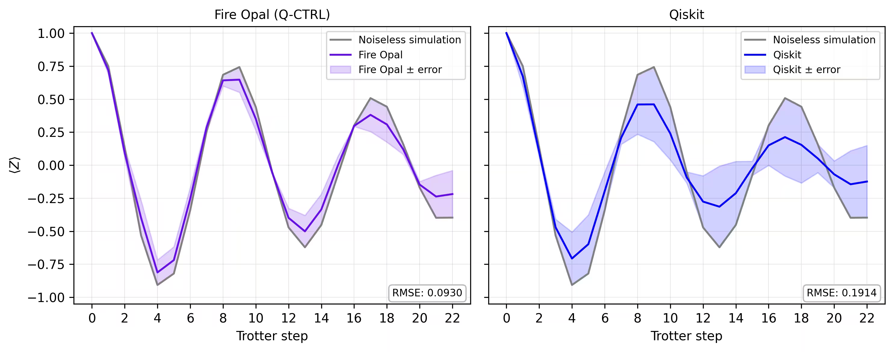
마지막으로, 시뮬레이터의 자화 곡선과 실제 하드웨어에서 얻은 결과를 비교합니다. 두 결과를 나란히 플롯하면 Fire Opal을 사용한 하드웨어 실행이 Trotter 단계 전반에 걸쳐 노이즈 없는 기준선과 얼마나 잘 일치하는지 확인할 수 있습니다.

def make_correlators(test_counts, nq, d_ind_tot):
    mz = np.empty((nq, d_ind_tot))
    for d_ind in range(d_ind_tot):
        counts = test_counts[d_ind]
        for i in range(nq):
            mz[i, d_ind] = z_expectation(counts, i)
    average_z = np.mean(mz, axis=0)
    return np.concatenate((np.array([1]), average_z), axis=0)

sim_exp = make_correlators(sim_counts[0:22], nq=nq, d_ind_tot=22)
qiskit_exp = make_correlators(qiskit_counts[0:22], nq=nq, d_ind_tot=22)

qctrl_exp = [ev.data.evs for ev in result_qctrl[:]]
qctrl_exp_mean = np.concatenate(
    (np.array([1]), np.mean(qctrl_exp, axis=1)), axis=0
)

def make_expectations_plot(
    sim_z,
    depths,
    exp_qctrl=None,
    exp_qctrl_error=None,
    exp_qiskit=None,
    exp_qiskit_error=None,
    plot_from=0,
    plot_upto=23,
):
    import numpy as np
    import matplotlib.pyplot as plt

    depth_ticks = [0, 2, 4, 6, 8, 10, 12, 14, 16, 18, 20, 22]

    d = np.asarray(depths)[plot_from:plot_upto]
    sim = np.asarray(sim_z)[plot_from:plot_upto]

    qk = (
        None
        if exp_qiskit is None
        else np.asarray(exp_qiskit)[plot_from:plot_upto]
    )
    qc = (
        None
        if exp_qctrl is None
        else np.asarray(exp_qctrl)[plot_from:plot_upto]
    )

    qk_err = (
        None
        if exp_qiskit_error is None
        else np.asarray(exp_qiskit_error)[plot_from:plot_upto]
    )
    qc_err = (
        None
        if exp_qctrl_error is None
        else np.asarray(exp_qctrl_error)[plot_from:plot_upto]
    )

    # ---- helper(s) ----
    def rmse(a, b):
        if a is None or b is None:
            return None
        a = np.asarray(a, dtype=float)
        b = np.asarray(b, dtype=float)
        mask = np.isfinite(a) & np.isfinite(b)
        if not np.any(mask):
            return None
        diff = a[mask] - b[mask]
        return float(np.sqrt(np.mean(diff**2)))

    def plot_panel(ax, method_y, method_err, color, label, band_color=None):
        # Noiseless reference
        ax.plot(d, sim, color="grey", label="Noiseless simulation")

        # Method line + band
        if method_y is not None:
            ax.plot(d, method_y, color=color, label=label)
            if method_err is not None:
                lo = np.clip(method_y - method_err, -1.05, 1.05)
                hi = np.clip(method_y + method_err, -1.05, 1.05)
                ax.fill_between(
                    d,
                    lo,
                    hi,
                    alpha=0.18,
                    color=band_color if band_color else color,
                    label=f"{label} ± error",
                )
        else:
            ax.text(
                0.5,
                0.5,
                "No data",
                transform=ax.transAxes,
                ha="center",
                va="center",
                fontsize=10,
                color="0.4",
            )

        # RMSE box (vs sim)
        r = rmse(method_y, sim)
        if r is not None:
            ax.text(
                0.98,
                0.02,
                f"RMSE: {r:.4f}",
                transform=ax.transAxes,
                va="bottom",
                ha="right",
                fontsize=8,
                bbox=dict(
                    boxstyle="round,pad=0.35", fc="white", ec="0.7", alpha=0.9
                ),
            )
        # Axes
        ax.set_xticks(depth_ticks)
        ax.set_ylim(-1.05, 1.05)
        ax.grid(True, which="both", linewidth=0.4, alpha=0.4)
        ax.set_axisbelow(True)
        ax.legend(prop={"size": 8}, loc="best")

    fig, axes = plt.subplots(1, 2, figsize=(10, 4), dpi=300, sharey=True)

    axes[0].set_title("Fire Opal (Q-CTRL)", fontsize=10)
    plot_panel(
        axes[0],
        qc,
        qc_err,
        color="#680CE9",
        label="Fire Opal",
        band_color="#680CE9",
    )
    axes[0].set_xlabel("Trotter step")
    axes[0].set_ylabel(r"$\langle Z \rangle$")
    axes[1].set_title("Qiskit", fontsize=10)
    plot_panel(
        axes[1], qk, qk_err, color="blue", label="Qiskit", band_color="blue"
    )
    axes[1].set_xlabel("Trotter step")

    plt.tight_layout()
    plt.show()

depths = list(range(d_ind_tot + 1))
errors = np.abs(np.array(qctrl_exp_mean) - np.array(sim_exp))

errors_qiskit = np.abs(np.array(qiskit_exp) - np.array(sim_exp))

make_expectations_plot(
    sim_exp,
    depths,
    exp_qctrl=qctrl_exp_mean,
    exp_qctrl_error=errors,
    exp_qiskit=qiskit_exp,
    exp_qiskit_error=errors_qiskit,
)

참고 문헌

[1] 그래프 채색. Wikipedia. 2025년 9월 15일 검색, https://en.wikipedia.org/wiki/Graph_coloring

튜토리얼 설문조사

이 튜토리얼에 대한 피드백을 남겨 주세요. 여러분의 의견은 콘텐츠 품질과 사용자 경험 개선에 큰 도움이 됩니다.

설문조사 링크

Note: This survey is provided by IBM Quantum and relates to the original English content. To give feedback on doQumentation's website, translations, or code execution, please open a GitHub issue.