반복 코드
사용 예상 시간: Heron 프로세서에서 10초 미만 (참고: 이는 추정치일 뿐이며, 실제 실행 시간은 다를 수 있습니다.)
학습 목표
-
동적 회로를 사용하여 비트 반전 오류 정정 코드를 구현하는 방법
-
인코딩된 정보를 파괴하지 않고 양자 오류를 감지하기 위해 안정자(stabilizer)를 측정하는 방법
-
보정된 결과와 보정되지 않은 결과를 비교하여 양자 오류 정정의 성능을 평가하는 방법
필수 조건
배경
실시간 양자 오류 정정(QEC)을 구현하려면, 측정 결과에 따라 양자 게이트를 조건부로 실행할 수 있도록 실행 중에 양자 프로그램의 흐름을 동적으로 제어할 수 있어야 합니다. 이 튜토리얼은 비트 반전 코드(bit-flip code)를 실행하며, 이는 매우 간단한 형태의 QEC입니다. 인코딩된 Qubit을 단일 비트 반전 오류로부터 보호할 수 있는 동적 양자 Circuit을 시연하고, 비트 반전 코드의 성능을 평가합니다.
추가 앤실라(ancilla) Qubit과 얽힘을 활용하여 인코딩된 양자 정보를 변환하지 않으면서도 발생했을 수 있는 특정 종류의 오류를 알려주는 *스태빌라이저(stabilizer)*를 측정할 수 있습니다. 양자 스태빌라이저 코드는 개의 논리 Qubit을 개의 물리 Qubit으로 인코딩합니다. 스태빌라이저 코드는 파울리 군 에 서포트(support)를 갖는, 즉 파울리 연산자로 구성된 이산 오류 집합을 정정하는 데 주로 중점을 둡니다.
이 튜토리얼에서는 간단한 양자 메모리 실험을 사용하여 비트 플립 코드를 시연합니다. 인코딩된 큐비트를 논리 상태 로 준비한 다음, 여러 사이클의 유휴 시간(오류를 축적하기 위해)을 구현하고 이어서 오류 검출 및 정정을 수행합니다. 그런 다음 사이클 수(시간)에 따른 논리적 오류 확률을 정량화하는데, 여기서 논리적 오류 확률은 최종 측정 후 큐비트가 을 복구하지 못하는 상태에서 발견될 확률입니다(구체적으로, 오류에 해당하는 상태는 , , , 입니다).
인코딩되지 않은 개별 큐비트의 오류율과 시간에 따른 오류율을 비교하고, 또한 최종 측정 후에만 오류를 검출하고 정정하되 회로 실행 중에는 동적으로 정정하지 않는 반복 코드의 사용과도 비교할 것입니다.
참고: 반복 코드는 비트 플립 오류의 정정만 허용하므로 완전한 오류 정정 코드가 아닙니다. 그러나 단순성 때문에 양자 컴퓨터에서 오류 정정을 구현하는 방법을 보여주기에 좋은 출발점입니다. 아래의 메모리 실험은 단일 유형의 오류(이 으로 붕괴하는 것)만 테스트하며, 기술적으로는 고전 정보의 보호만 시연합니다.
요구 사항
이 튜토리얼을 시작하기 전에 다음이 설치되어 있는지 확인하세요:
-
Qiskit SDK v2.0 이상, 시각화 지원 포함
-
Qiskit Runtime v0.40 이상 (
pip install qiskit-ibm-runtime)
설정
# Added by doQumentation — required packages for this notebook
!pip install -q matplotlib numpy qiskit qiskit-ibm-runtime scipy seaborn
import numpy as np
import seaborn as sns
import matplotlib.pyplot as plt
from scipy.optimize import curve_fit

sns.set()
plt.rc("xtick", labelsize=20)
plt.rc("ytick", labelsize=20)
plt.rc("lines", linewidth=3)
plt.rc("font", size=20)
plt.rc("legend", fontsize="large")
plt.rc("axes", labelsize=20)
plt.rcParams["figure.figsize"] = 15, 6
plt.rcParams["legend.title_fontsize"] = 25
# Qiskit imports
from qiskit import (
    QuantumCircuit,
    QuantumRegister,
    ClassicalRegister,
)

# qiskit-ibm-runtime
from qiskit_ibm_runtime import QiskitRuntimeService, SamplerV2 as Sampler
from qiskit_ibm_runtime.circuit import MidCircuitMeasure

service = QiskitRuntimeService()
소규모 시뮬레이터 예제
이 실험의 목표는 진폭 감쇠와 같은 실제 하드웨어 노이즈 하에서 논리적 큐비트의 수명을 측정하는 것이므로, 이 단계는 생략하겠습니다. 노이즈가 없는 시뮬레이터는 검출하고 정정할 오류가 없기 때문입니다.
대규모 하드웨어 예제
1단계. 고전적 입력을 양자 문제로 변환
백엔드 선택
회로 실행 중 오류를 검출하려면 MidCircuitMeasure 방법에 액세스할 수 있는 백엔드를 선택해야 합니다(문서 참조).
# You can see all backends that support mid-circuit measurements by running the following code.
service.backends(filters=lambda b: "measure_2" in b.supported_instructions)
[<IBMBackend('ibm_pittsburgh')>,
 <IBMBackend('ibm_boston')>,
 <IBMBackend('ibm_kingston')>]
# Choose the least busy backend that supports mid-circuit measurements (`measure_2`).

backend = service.least_busy(
    filters=lambda b: "measure_2" in b.supported_instructions,
    operational=True,
    simulator=False,
    dynamic_circuits=True,
)
# backend = service.backend(backend_name) # alternatively, you could choose a specific backend
print(backend.name)
ibm_boston
여러 라운드의 오류 검출 및 정정을 구현하는 일련의 비트 플립 안정자 회로 구축
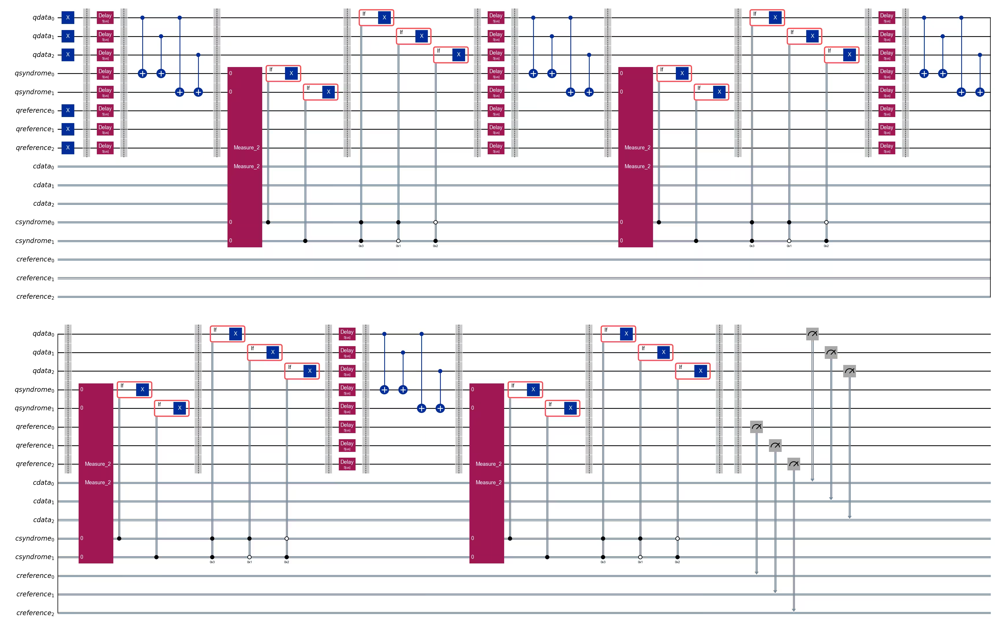
비트 반전 코드는 스태빌라이저 코드의 가장 간단한 예 중 하나입니다. 이 코드는 인코딩 qubit 중 어느 하나에 대한 단일 비트 반전(X) 오류로부터 상태를 보호합니다. 및 으로 매핑하는 비트 반전 오류 의 작용을 고려하면, 가 됩니다. 이 코드는 다섯 개의 Qubit이 필요합니다: 세 개는 보호된 상태("데이터 qubit")를 인코딩하는 데 사용되고, 나머지 두 개는 스태빌라이저 측정 앤실라로 사용됩니다.
아래에서는 (1) 데이터 큐비트를 논리 상태로 준비한 다음, (2) 지연 후 오류 정정(신드롬 큐비트 재설정 포함)을 수행하는 여러 사이클을 실행하고, (3) 데이터 큐비트의 상태를 읽어내는 회로를 만들 것입니다.
또한 상태로 준비하고, 유휴 상태로 두었다가 읽어내는 세 개의 참조 큐비트를 포함하여 오류 정정을 사용하지 않은 상태의 수명도 테스트할 것입니다.
def build_qc(
    qreg_data,
    qreg_syndrome,
    creg_data,
    creg_syndrome,
    qreg_ref=None,
    creg_ref=None,
):
    """Build a typical error correction circuit"""
    if qreg_ref:
        return QuantumCircuit(
            qreg_data,
            qreg_syndrome,
            creg_data,
            creg_syndrome,
            qreg_ref,
            creg_ref,
        )
    else:
        return QuantumCircuit(
            qreg_data, qreg_syndrome, creg_data, creg_syndrome
        )

def encode_bit_flip(circuit, qreg_data, qreg_ref=None) -> QuantumCircuit:
    """Encode bit-flip. This is done by simply adding a cx"""

    for q in qreg_data:
        circuit.x(q)

    if qreg_ref:
        for q in qreg_ref:
            circuit.x(q)

    circuit.barrier()

    return circuit

def measure_syndrome_bit(
    circuit, qreg_data, qreg_syndrome, creg_syndrome, qreg_ref=None
):
    """
    Measure the syndrome by measuring the parity.
    We reset our ancilla qubits after measuring the stabilizer
    so we can reuse them for repeated stabilizer measurements.
    Because we have already observed the state of the qubit,
    we can write the conditional reset protocol directly to
    avoid another round of qubit measurement if we used
    the `reset` instruction.
    """
    circuit.cx(qreg_data[0], qreg_syndrome[0])
    circuit.cx(qreg_data[1], qreg_syndrome[0])
    circuit.cx(qreg_data[0], qreg_syndrome[1])
    circuit.cx(qreg_data[2], qreg_syndrome[1])
    circuit.barrier()

    for q_measure, c_measure in zip(qreg_syndrome, creg_syndrome):
        circuit.append(MidCircuitMeasure(), [q_measure], [c_measure])

    with circuit.if_test((creg_syndrome[0], 1)):
        circuit.x(qreg_syndrome[0])
    with circuit.if_test((creg_syndrome[1], 1)):
        circuit.x(qreg_syndrome[1])

    circuit.barrier()
    return circuit

def apply_correction_bit(circuit, qreg_data, creg_syndrome):
    """We can detect where an error occurred and correct our state"""
    with circuit.if_test((creg_syndrome, 3)):
        circuit.x(qreg_data[0])
    with circuit.if_test((creg_syndrome, 1)):
        circuit.x(qreg_data[1])
    with circuit.if_test((creg_syndrome, 2)):
        circuit.x(qreg_data[2])
    circuit.barrier()
    return circuit

def apply_final_readout(
    circuit, qreg_data, creg_data, qreg_ref=None, creg_ref=None
):
    """Read out the final measurements"""

    circuit.barrier()
    if qreg_ref:
        circuit.measure(qreg_ref, creg_ref)
    circuit.measure(qreg_data, creg_data)

    return circuit
def build_error_correction_sequence(
    num_cycles, cycles_per_circuit, nq_ref=3, delay=None
) -> QuantumCircuit:
    circuits = []
    reps = []

    qreg_data = QuantumRegister(3, name="qdata")
    qreg_syndrome = QuantumRegister(2, name="qsyndrome")
    creg_data = ClassicalRegister(3, name="cdata")
    creg_syndrome = ClassicalRegister(2, name="csyndrome")
    qreg_ref = QuantumRegister(nq_ref, name="qreference")
    creg_ref = ClassicalRegister(nq_ref, name="creference")

    circuit = build_qc(
        qreg_data,
        qreg_syndrome,
        creg_data,
        creg_syndrome,
        qreg_ref=qreg_ref,
        creg_ref=creg_ref,
    )
    circuit = encode_bit_flip(circuit, qreg_data, qreg_ref=qreg_ref)

    circuit_n = circuit.copy()
    circuit_n = apply_final_readout(
        circuit_n, qreg_data, creg_data, qreg_ref=qreg_ref, creg_ref=creg_ref
    )
    circuits.append(circuit_n)
    reps.append(0)

    for i in range(1, num_cycles + 1):
        if delay:
            circuit.delay(delay, unit="us")
            circuit.barrier()
        circuit = measure_syndrome_bit(
            circuit,
            qreg_data,
            qreg_syndrome,
            creg_syndrome,
            qreg_ref=qreg_ref,
        )
        circuit = apply_correction_bit(circuit, qreg_data, creg_syndrome)
        circuit_n = circuit.copy()
        if i % cycles_per_circuit == 0:
            circuit_n = apply_final_readout(
                circuit_n,
                qreg_data,
                creg_data,
                qreg_ref=qreg_ref,
                creg_ref=creg_ref,
            )
            circuits.append(circuit_n)
            reps.append(i)

    return circuits, np.array(reps)

num_cycles = 40
cycles_per_circuit = 4
nq_ref = 3
circuits, rep_array = build_error_correction_sequence(
    num_cycles, cycles_per_circuit, nq_ref=3, delay=5
)
circuits[1].draw(output="mpl", cregbundle=False, fold=50)
Step 2: 양자 하드웨어 실행을 위한 문제 최적화
총 작업 실행 시간을 줄이기 위해, Qiskit 프리미티브는 대상 시스템이 지원하는 명령어 및 연결성에 맞는 Circuit과 옵저버블만 허용합니다(명령어 집합 아키텍처(ISA) Circuit 및 옵저버블이라고 합니다). 트랜스파일에 대해 더 알아보기.
ISA Circuit 생성
먼저 최적화 수준 3의 사전 설정 패스 매니저를 사용하여 회로 중 가장 긴 회로를 트랜스파일함으로써 초기 레이아웃(즉, 회로를 매핑할 물리적 큐비트의 선택)을 찾는 것부터 시작하겠습니다.
from qiskit.transpiler.preset_passmanagers import generate_preset_pass_manager

pm = generate_preset_pass_manager(backend=backend, optimization_level=3)
isa_circuit_ref = pm.run(circuits[-1])
init_layout = isa_circuit_ref.layout.initial_index_layout(
    filter_ancillas=True
)
print(init_layout)
[56, 44, 62, 43, 63, 22, 48, 67]
논리적 양자 메모리와 비교할 참조 큐비트의 경우, 진폭 감쇠 결맞음 시간() 측면에서 사용 가능한 최고의 큐비트로 선택하겠습니다.
# get all qubits ordered by T1
t1_data = []
for i in range(backend.num_qubits):
    try:
        t1_us = backend.properties().t1(i) * 1e6
    except Exception:
        t1_us = 0.0
    t1_data.append((i, t1_us))

t1_data_sorted = sorted(t1_data, key=lambda x: x[1], reverse=True)

# exclude the qubits we have already mapped the error correcting code to
t1_data_sorted = [
    t1_data for t1_data in t1_data_sorted if t1_data[0] not in init_layout[:5]
]

# use the best qubits in terms of T1 for the reference qubits
init_layout = init_layout[:5] + [t1_data[0] for t1_data in t1_data_sorted[:3]]
print(init_layout)
[56, 44, 62, 43, 63, 143, 131, 31]
# These are the resulting T1 times
properties = backend.properties()
print("Amplitude damping decoherence times for code data qubits:")
for q in init_layout[:3]:
    t1 = properties.t1(q)
    print(f"qubit {q}: T1 = {t1 * 1e6:.0f} mus")

print("\nAmplitude damping decoherence times for reference qubits:")
for q in init_layout[-3:]:
    t1 = properties.t1(q)
    print(f"qubit {q}: T1 = {t1 * 1e6:.0f} mus")
Amplitude damping decoherence times code data qubits:
qubit 56: T1 = 322 mus
qubit 44: T1 = 263 mus
qubit 62: T1 = 290 mus

Amplitude damping decoherence times reference qubits:
qubit 143: T1 = 442 mus
qubit 131: T1 = 410 mus
qubit 31: T1 = 401 mus
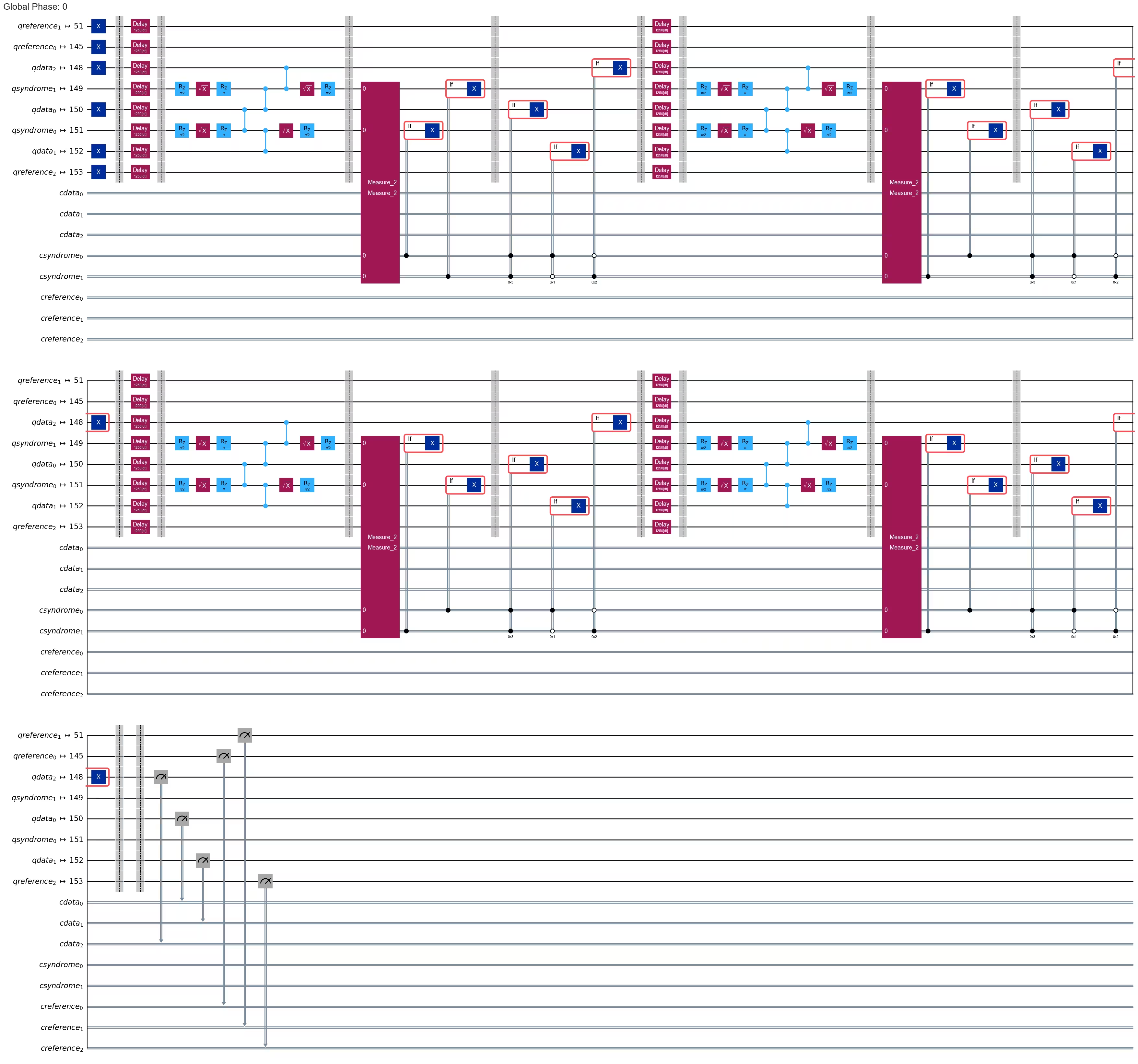
# now we transpile all circuits to this initial layout; this way each circuit is run on the same qubits and we can make a fair comparison
pm = generate_preset_pass_manager(
    backend=backend,
    optimization_level=3,
    initial_layout=init_layout,
)
isa_circuits = pm.run(circuits)
isa_circuits[1].draw("mpl", cregbundle=False, fold=50)
3단계. Qiskit 프리미티브를 사용하여 실행
sampler = Sampler(mode=backend)

sampler.options.environment.job_tags = ["TUT-REPCODE"]
sampler.options.max_execution_time = 600  # this workload is expected to be under 10s, but it is generally a good habit to set a max execution time (here 600s = 10m)
job = sampler.run(isa_circuits, shots=1000)
print(job.job_id())
job.status()
'DONE'
4단계: 후처리하고 원하는 고전적 형식으로 결과 반환
이제 3큐비트 반복 코드를 사용하는 논리적 메모리와 인코딩되지 않은 개별 참조 큐비트 간의 시간 대비 오류율을 비교하겠습니다.
results = job.result()
def correct_counts(counts_dict):
    """
    Corrects the measured logical qubit encoded in the repetition code using majority vote
    """

    result = {"000": 0, "111": 0}
    for bitstring, count in counts_dict.items():
        key = "111" if bitstring.count("1") > 1 else "000"
        result[key] += count
    return result

accuracy = []  # logical qubit
accuracies_ref = np.zeros(
    (len(results), nq_ref)
)  # accuracies on individual reference qubits

for n, pub_result in enumerate(results):
    # logical accuracy (one minus error probability) for active error correction with repetition code
    counts = pub_result.data.cdata.get_counts()
    shots = sum(counts.values())
    counts_corrected = correct_counts(counts)
    accuracy.append(counts_corrected.get("111", 0) / shots)

    # accuracy for individual physical reference qubits without any error correction
    for i in range(nq_ref):
        counts = pub_result.data.creference.slice_bits(i).get_counts()
        accuracies_ref[n, i] = counts.get("1", 0) / shots

accuracy = np.array(accuracy)
def error_proba_t1(N, t1):
    """
    Exponential fitting function for amplitude damping vs. number of cycles
    """

    t_cycle = 7.3e-6  # approximate time per cycle = 5 mus delay + 2.3 mus for error correction
    return 1 - np.exp(-t_cycle * N / t1)

fig, ax = plt.subplots(1, 1, figsize=(15, 5))
ax.plot(
    rep_array, (1.0 - accuracy) * 100.0, "ko-", linewidth=3, label="rep code"
)

for i in range(nq_ref):
    accuracy_1q = accuracies_ref[:, i]
    if i == 0:
        ax.plot(
            rep_array,
            (1.0 - accuracy_1q) * 100.0,
            "go-",
            linewidth=1,
            label="1q reference",
        )
    else:
        ax.plot(rep_array, (1.0 - accuracy_1q) * 100.0, "go-", linewidth=1)

params_bf, pcov = curve_fit(
    error_proba_t1, rep_array, 1.0 - accuracy, bounds=([0, 5e-3])
)
t1_bf = params_bf[0]
print(f"Best-fit effective T1 = {t1_bf * 1e6:.0f} us")
error_prob_bf = error_proba_t1(
    rep_array, t1_bf
)  # np.array([1 - np.exp(-t_cycle * nt/t1) for nt in rep_array])
ax.plot(rep_array, error_prob_bf * 100.0, "k--", linewidth=1)

ax.set_xlabel("error correction rounds")
ax.set_ylabel("error [%]")
ax.set_ylim(bottom=0)
ax.legend(fontsize=15);
Best-fit effective T1 = 1397 us
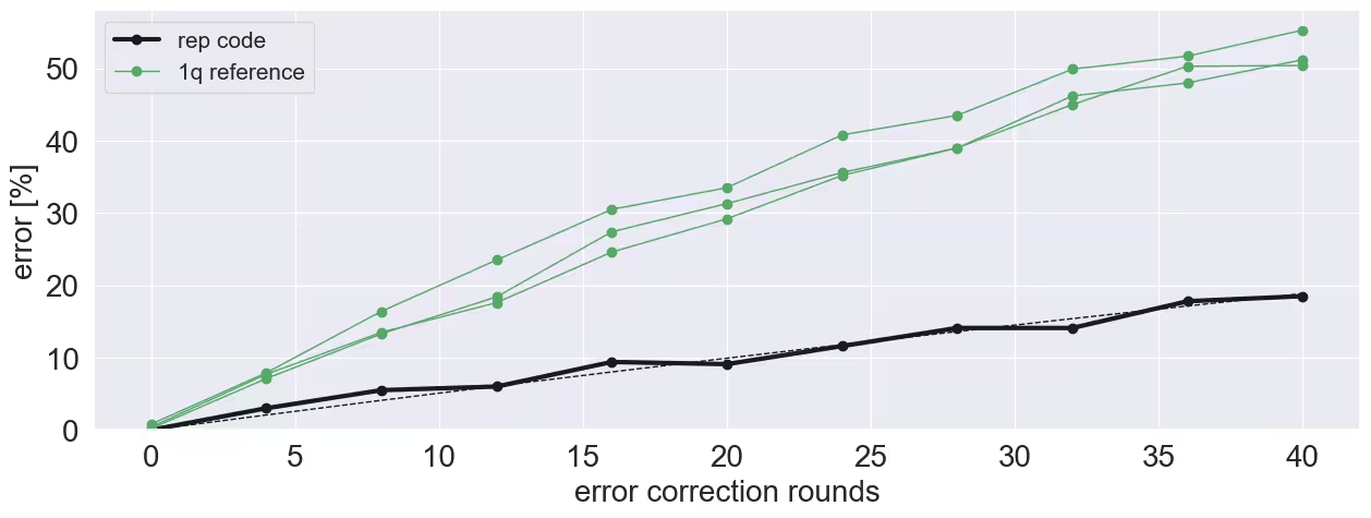
최고의 (인코딩되지 않은) 물리적 큐비트와 비교하더라도 상태의 향상된 수명을 명확히 볼 수 있습니다. 그러나 이 실험은 비트 플립이라는 한 가지 유형의 오류만 정정한다는 점을 명심하세요. 논리적 큐비트의 수명을 개선할 수 있을까요? 지연 시간을 최적화하거나 반복 코드의 크기를 이상으로 확장하는 등을 탐색해 볼 수 있습니다.
다음 단계
이 작업이 흥미로우셨다면 다음 자료에 관심이 있으실 수 있습니다:
-
양자 오류 정정의 기초 강좌 - 양자 오류 정정에 대해 자세히 알아보기
-
시공간 코드를 이용한 저오버헤드 오류 검출 튜토리얼 - Pauli 검사를 사용하여 오류를 검출하고 샘플을 사후 선택하는 방법 알아보기