Qubit 선택을 위한 실시간 벤치마킹
사용 시간 추정: Eagle r2 프로세서에서 약 4분 (참고: 이는 추정치이며 실제 실행 시간은 다를 수 있습니다.)
# Added by doQumentation — required packages for this notebook
!pip install -q matplotlib numpy qiskit qiskit-experiments qiskit-ibm-runtime rustworkx
# This cell is hidden from users – it disables some lint rules
# ruff: noqa: E722
배경
이 튜토리얼은 실시간 특성 실험을 실행하고 백엔드 속성을 업데이트하여 Circuit을 QPU의 물리적 Qubit에 매핑할 때 qubit 선택을 개선하는 방법을 설명합니다. QPU의 속성을 결정하는 데 사용되는 기본 특성 실험, Qiskit에서 이를 수행하는 방법, 그리고 이러한 실험을 바탕으로 QPU를 나타내는 백엔드 객체에 저장된 속성을 업데이트하는 방법을 배울 수 있습니다.
QPU가 보고하는 속성은 하루에 한 번 업데이트되지만, 시스템은 업데이트 간격보다 빠르게 변동할 수 있습니다. 이는 패스 매니저의 Layout 단계에서 사용하는 qubit 선택 루틴의 신뢰성에 영향을 줄 수 있는데, 보고된 속성이 QPU의 현재 상태를 반영하지 못할 수 있기 때문입니다. 이러한 이유로 특성 실험에 일부 QPU 시간을 할애하는 것이 가치 있을 수 있으며, 이를 통해 Layout 루틴에서 사용하는 QPU 속성을 업데이트할 수 있습니다.
요구 사항
이 튜토리얼을 시작하기 전에 다음이 설치되어 있는지 확인하세요:
- Qiskit SDK v2.0 이상 (시각화 지원 포함)
- Qiskit Runtime v0.40 이상 (
pip install qiskit-ibm-runtime) - Qiskit Experiments v0.12 이상 (
pip install qiskit-experiments) - Rustworkx 그래프 라이브러리 (
pip install rustworkx)
설정
from qiskit_ibm_runtime import SamplerV2
from qiskit.transpiler import generate_preset_pass_manager
from qiskit.quantum_info import hellinger_fidelity
from qiskit.transpiler import InstructionProperties

from qiskit_experiments.library import (
    T1,
    T2Hahn,
    LocalReadoutError,
    StandardRB,
)
from qiskit_experiments.framework import BatchExperiment, ParallelExperiment

from qiskit_ibm_runtime import QiskitRuntimeService
from qiskit_ibm_runtime import Session

from datetime import datetime
from collections import defaultdict
import numpy as np
import rustworkx
import matplotlib.pyplot as plt
import copy
Step 1: 고전 입력을 양자 문제로 매핑하기
성능 차이를 벤치마킹하기 위해 다양한 길이의 선형 체인 전반에 걸쳐 Bell 상태를 준비하는 Circuit을 고려합니다. 체인의 양 끝에서 Bell 상태의 충실도를 측정합니다.
from qiskit import QuantumCircuit

ideal_dist = {"00": 0.5, "11": 0.5}

num_qubits_list = [10, 20, 30, 40, 50, 60, 70, 80, 90, 100, 110, 120, 127]
circuits = []
for num_qubits in num_qubits_list:
    circuit = QuantumCircuit(num_qubits, 2)
    circuit.h(0)
    for i in range(num_qubits - 1):
        circuit.cx(i, i + 1)
    circuit.barrier()
    circuit.measure(0, 0)
    circuit.measure(num_qubits - 1, 1)
    circuits.append(circuit)

circuits[-1].draw(output="mpl", style="clifford", fold=-1)


백엔드 및 커플링 맵 설정
먼저 백엔드를 선택합니다.
# To run on hardware, select the backend with the fewest number of jobs in the queue
service = QiskitRuntimeService()
backend = service.least_busy(
    operational=True, simulator=False, min_num_qubits=127
)

qubits = list(range(backend.num_qubits))
그런 다음 커플링 맵을 가져옵니다.
coupling_graph = backend.coupling_map.graph.to_undirected(multigraph=False)

# Get unidirectional coupling map
one_dir_coupling_map = coupling_graph.edge_list()
가능한 한 많은 2-Qubit Gate를 동시에 벤치마킹하기 위해 커플링 맵을 layered_coupling_map으로 분리합니다. 이 객체는 레이어 목록을 포함하며, 각 레이어는 동시에 2-Qubit Gate를 실행할 수 있는 엣지 목록입니다. 이를 커플링 맵의 엣지 색칠이라고도 합니다.
# Get layered coupling map
edge_coloring = rustworkx.graph_bipartite_edge_color(coupling_graph)
layered_coupling_map = defaultdict(list)
for edge_idx, color in edge_coloring.items():
    layered_coupling_map[color].append(
        coupling_graph.get_edge_endpoints_by_index(edge_idx)
    )
layered_coupling_map = [
    sorted(layered_coupling_map[i])
    for i in sorted(layered_coupling_map.keys())
]
특성 실험
QPU에서 Qubit의 주요 속성을 특성화하기 위해 일련의 실험이 사용됩니다. 이는 , , 읽기 오류, 단일 qubit 및 2-Qubit Gate 오류입니다. 이러한 속성이 무엇인지 간략하게 설명하고, 이를 특성화하는 데 사용되는 qiskit-experiments 패키지의 실험을 소개합니다.
T1
은 진폭 감쇠 디코히어런스 과정으로 인해 들뜬 Qubit이 바닥 상태로 떨어지는 데 걸리는 특성 시간입니다. 실험에서는 지연 후 들뜬 Qubit을 측정합니다. 지연 시간이 길수록 Qubit이 바닥 상태로 떨어질 가능성이 높아집니다. 실험의 목표는 Qubit이 바닥 상태로 향하는 감쇠율을 특성화하는 것입니다.
T2
는 단일 Qubit의 블로흐 벡터가 XY 평면에 투영된 값이 위상 이완 디코히어런스 과정으로 인해 초기 진폭의 약 37% ()로 떨어지는 데 필요한 시간을 나타냅니다. Hahn Echo 실험에서 이 감쇠 속도를 추정할 수 있습니다.
상태 준비 및 측정(SPAM) 오류 특성화
SPAM 오류 특성화 실험에서 Qubit은 특정 상태( 또는 )로 준비되고 측정됩니다. 준비된 상태와 다른 상태가 측정될 확률이 오류 확률을 나타냅니다.
단일 qubit 및 2-Qubit 무작위 벤치마킹
무작위 벤치마킹(RB)은 양자 프로세서의 오류율을 특성화하는 널리 사용되는 프로토콜입니다. RB 실험은 주어진 Qubit에 대해 계산된 유니터리가 항등 연산이 되도록 무작위 클리포드 Circuit을 생성하는 것으로 구성됩니다. Circuit을 실행한 후 오류(즉, 바닥 상태와 다른 출력)가 발생한 샷 수를 계산하고, 이 데이터로부터 클리포드당 오류(Error Per Clifford)를 계산하여 양자 장치의 오류 추정값을 도출합니다.
# Create T1 experiments on all qubit in parallel
t1_exp = ParallelExperiment(
    [
        T1(
            physical_qubits=[qubit],
            delays=[1e-6, 20e-6, 40e-6, 80e-6, 200e-6, 400e-6],
        )
        for qubit in qubits
    ],
    backend,
    analysis=None,
)

# Create T2-Hahn experiments on all qubit in parallel
t2_exp = ParallelExperiment(
    [
        T2Hahn(
            physical_qubits=[qubit],
            delays=[1e-6, 20e-6, 40e-6, 80e-6, 200e-6, 400e-6],
        )
        for qubit in qubits
    ],
    backend,
    analysis=None,
)

# Create readout experiments on all qubit in parallel
readout_exp = LocalReadoutError(qubits)

# Create single-qubit RB experiments on all qubit in parallel
singleq_rb_exp = ParallelExperiment(
    [
        StandardRB(
            physical_qubits=[qubit], lengths=[10, 100, 500], num_samples=10
        )
        for qubit in qubits
    ],
    backend,
    analysis=None,
)

# Create two-qubit RB experiments on the three layers of disjoint edges of the heavy-hex
twoq_rb_exp_batched = BatchExperiment(
    [
        ParallelExperiment(
            [
                StandardRB(
                    physical_qubits=pair,
                    lengths=[10, 50, 100],
                    num_samples=10,
                )
                for pair in layer
            ],
            backend,
            analysis=None,
        )
        for layer in layered_coupling_map
    ],
    backend,
    flatten_results=True,
    analysis=None,
)
시간에 따른 QPU 속성
시간에 따른 QPU 속성(아래에서 단일 주를 고려합니다)을 살펴보면, 이러한 속성이 하루 단위로 어떻게 변동할 수 있는지 알 수 있습니다. 하루 이내에도 소폭의 변동이 발생할 수 있습니다. 이러한 시나리오에서는 (하루에 한 번 업데이트되는) 보고된 속성이 QPU의 현재 상태를 정확하게 반영하지 못합니다. 또한 작업이 로컬에서 트랜스파일(현재 보고된 속성 사용)되고 제출되었지만 나중에(몇 분 또는 며칠 후) 실행되는 경우, 트랜스파일 단계에서 qubit 선택에 오래된 속성을 사용할 위험이 있습니다. 이는 실행 시점에 QPU에 대한 최신 정보를 보유하는 것의 중요성을 강조합니다. 먼저 특정 시간 범위에 걸쳐 속성을 가져옵니다.
instruction_2q_name = "cz"  # set the name of the default 2q of the device
errors_list = []
for day_idx in range(10, 17):
    calibrations_time = datetime(
        year=2025, month=8, day=day_idx, hour=0, minute=0, second=0
    )
    targer_hist = backend.target_history(datetime=calibrations_time)

    t1_dict, t2_dict = {}, {}
    for qubit in range(targer_hist.num_qubits):
        t1_dict[qubit] = targer_hist.qubit_properties[qubit].t1
        t2_dict[qubit] = targer_hist.qubit_properties[qubit].t2

    errors_dict = {
        "1q": targer_hist["sx"],
        "2q": targer_hist[f"{instruction_2q_name}"],
        "spam": targer_hist["measure"],
        "t1": t1_dict,
        "t2": t2_dict,
    }

    errors_list.append(errors_dict)
그런 다음 값을 플롯합니다.
fig, axs = plt.subplots(5, 1, figsize=(10, 20), sharex=False)

# Plot for T1 values
for qubit in range(targer_hist.num_qubits):
    t1s = []
    for errors_dict in errors_list:
        t1_dict = errors_dict["t1"]
        try:
            t1s.append(t1_dict[qubit] / 1e-6)
        except:
            print(f"missing t1 data for qubit {qubit}")

    axs[0].plot(t1s)

axs[0].set_title("T1")
axs[0].set_ylabel(r"Time ($\mu s$)")
axs[0].set_xlabel("Days")

# Plot for T2 values
for qubit in range(targer_hist.num_qubits):
    t2s = []
    for errors_dict in errors_list:
        t2_dict = errors_dict["t2"]
        try:
            t2s.append(t2_dict[qubit] / 1e-6)
        except:
            print(f"missing t2 data for qubit {qubit}")

    axs[1].plot(t2s)

axs[1].set_title("T2")
axs[1].set_ylabel(r"Time ($\mu s$)")
axs[1].set_xlabel("Days")

# Plot SPAM values
for qubit in range(targer_hist.num_qubits):
    spams = []
    for errors_dict in errors_list:
        spam_dict = errors_dict["spam"]
        spams.append(spam_dict[tuple([qubit])].error)

    axs[2].plot(spams)

axs[2].set_title("SPAM Errors")
axs[2].set_ylabel("Error Rate")
axs[2].set_xlabel("Days")

# Plot 1Q Gate Errors
for qubit in range(targer_hist.num_qubits):
    oneq_gates = []
    for errors_dict in errors_list:
        oneq_gate_dict = errors_dict["1q"]
        oneq_gates.append(oneq_gate_dict[tuple([qubit])].error)

    axs[3].plot(oneq_gates)

axs[3].set_title("1Q Gate Errors")
axs[3].set_ylabel("Error Rate")
axs[3].set_xlabel("Days")

# Plot 2Q Gate Errors
for pair in one_dir_coupling_map:
    twoq_gates = []
    for errors_dict in errors_list:
        twoq_gate_dict = errors_dict["2q"]
        twoq_gates.append(twoq_gate_dict[pair].error)

    axs[4].plot(twoq_gates)

axs[4].set_title("2Q Gate Errors")
axs[4].set_ylabel("Error Rate")
axs[4].set_xlabel("Days")

plt.subplots_adjust(hspace=0.5)
plt.show()
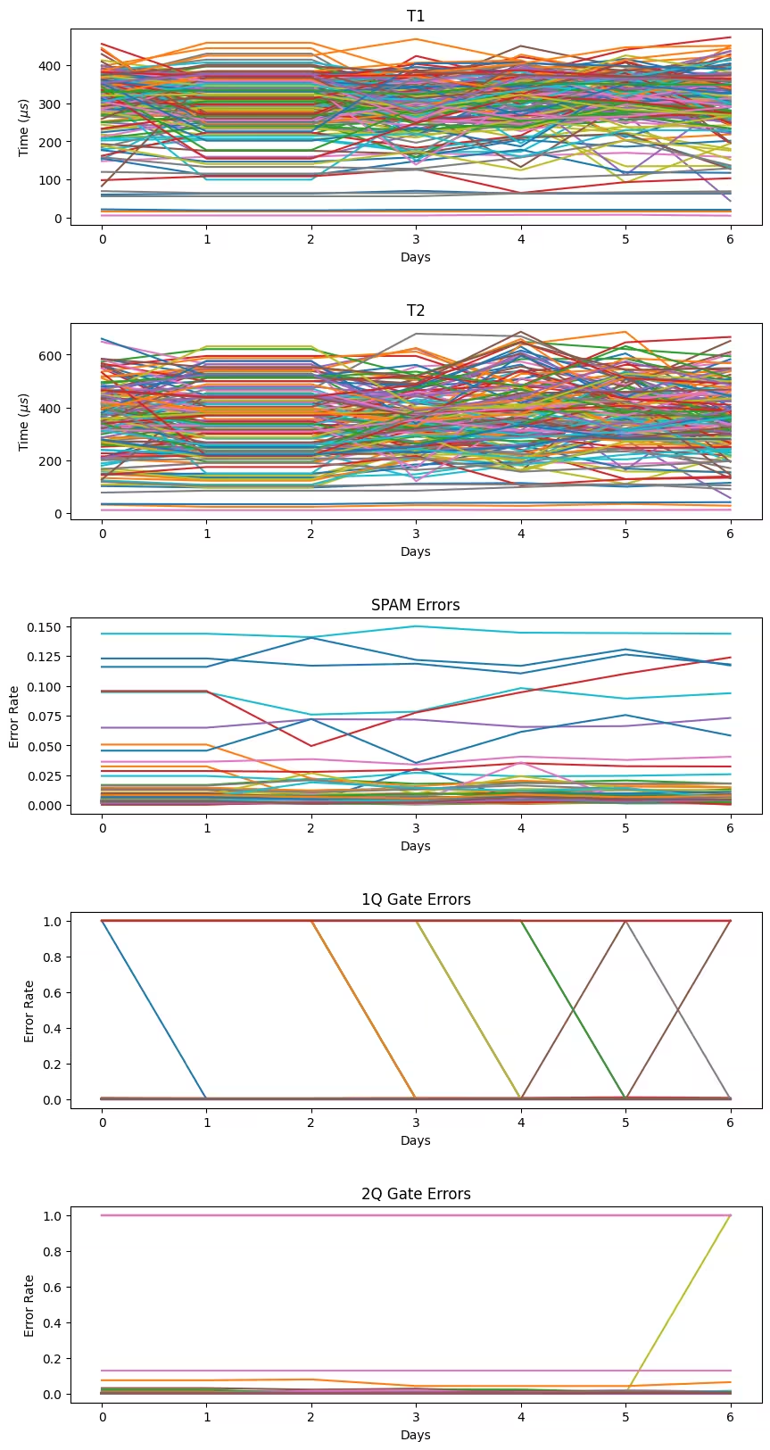
며칠에 걸쳐 일부 qubit 속성이 상당히 변할 수 있음을 확인할 수 있습니다. 이는 실험에서 가장 성능이 좋은 Qubit을 선택하기 위해 QPU 상태에 대한 최신 정보를 보유하는 것의 중요성을 잘 보여줍니다.
Step 2: 양자 하드웨어 실행을 위한 문제 최적화
이 튜토리얼에서는 Circuit 또는 연산자에 대한 최적화를 수행하지 않습니다.
Step 3: Qiskit 프리미티브를 사용하여 실행
기본 qubit 선택으로 양자 Circuit 실행
성능의 기준 결과로서, 요청된 Backend 속성에 따라 선택된 기본 Qubit을 사용하여 QPU에서 양자 Circuit을 실행합니다. optimization_level = 3을 사용합니다. 이 설정은 가장 고급 트랜스파일 최적화를 포함하며, 실행에 가장 성능이 좋은 Qubit을 선택하기 위해 연산 오류와 같은 대상 속성을 활용합니다.
pm = generate_preset_pass_manager(target=backend.target, optimization_level=3)
isa_circuits = pm.run(circuits)
initial_qubits = [
    [
        idx
        for idx, qb in circuit.layout.initial_layout.get_physical_bits().items()
        if qb._register.name != "ancilla"
    ]
    for circuit in isa_circuits
]
실시간 qubit 선택으로 양자 Circuit 실행
이 섹션에서는 최적의 결과를 위해 QPU의 qubit 속성에 대한 최신 정보를 갖추는 것이 얼마나 중요한지 살펴봅니다. 먼저, QPU 특성화 실험의 전체 집합(, , SPAM, 단일 qubit RB 및 이중 qubit RB)을 수행하여 Backend 속성을 업데이트하는 데 활용합니다. 이를 통해 Pass Manager가 QPU에 대한 최신 정보를 기반으로 실행할 Qubit을 선택하여 실행 성능을 향상시킬 수 있습니다. 다음으로, Bell pair Circuit을 실행하고 업데이트된 QPU 속성으로 Qubit을 선택한 경우의 충실도와 기본 보고된 속성으로 Qubit을 선택한 경우의 충실도를 비교합니다.
일부 특성화 실험은 피팅 루틴이 측정된 데이터에 곡선을 맞출 수 없을 때 실패할 수 있습니다. 이러한 실험에서 경고가 표시되면, 어떤 Qubit에서 어떤 특성화가 실패했는지 파악하고 실험 매개변수(예: , 시간이나 RB 실험의 길이 수)를 조정해 보세요.
# Prepare characterization experiments
batches = [t1_exp, t2_exp, readout_exp, singleq_rb_exp, twoq_rb_exp_batched]
batches_exp = BatchExperiment(batches, backend)  # , analysis=None)
run_options = {"shots": 1e3, "dynamic": False}

with Session(backend=backend) as session:
    sampler = SamplerV2(mode=session)

    # Run characterization experiments
    batches_exp_data = batches_exp.run(
        sampler=sampler, **run_options
    ).block_for_results()

    EPG_sx_result_list = batches_exp_data.analysis_results("EPG_sx")
    EPG_sx_result_q_indices = [
        result.device_components.index for result in EPG_sx_result_list
    ]
    EPG_x_result_list = batches_exp_data.analysis_results("EPG_x")
    EPG_x_result_q_indices = [
        result.device_components.index for result in EPG_x_result_list
    ]
    T1_result_list = batches_exp_data.analysis_results("T1")
    T1_result_q_indices = [
        result.device_components.index for result in T1_result_list
    ]

    T2_result_list = batches_exp_data.analysis_results("T2")
    T2_result_q_indices = [
        result.device_components.index for result in T2_result_list
    ]

    Readout_result_list = batches_exp_data.analysis_results(
        "Local Readout Mitigator"
    )

    EPG_2q_result_list = batches_exp_data.analysis_results(
        f"EPG_{instruction_2q_name}"
    )

    # Update target properties
    target = copy.deepcopy(backend.target)
    for i in range(target.num_qubits - 1):
        qarg = (i,)

        if qarg in EPG_sx_result_q_indices:
            target.update_instruction_properties(
                instruction="sx",
                qargs=qarg,
                properties=InstructionProperties(
                    error=EPG_sx_result_list[i].value.nominal_value
                ),
            )
        if qarg in EPG_x_result_q_indices:
            target.update_instruction_properties(
                instruction="x",
                qargs=qarg,
                properties=InstructionProperties(
                    error=EPG_x_result_list[i].value.nominal_value
                ),
            )

        err_mat = Readout_result_list.value.assignment_matrix(i)
        readout_assignment_error = (
            err_mat[0, 1] + err_mat[1, 0]
        ) / 2  # average readout error
        target.update_instruction_properties(
            instruction="measure",
            qargs=qarg,
            properties=InstructionProperties(error=readout_assignment_error),
        )

        if qarg in T1_result_q_indices:
            target.qubit_properties[i].t1 = T1_result_list[
                i
            ].value.nominal_value
        if qarg in T2_result_q_indices:
            target.qubit_properties[i].t2 = T2_result_list[
                i
            ].value.nominal_value

    for pair_idx, pair in enumerate(one_dir_coupling_map):
        qarg = tuple(pair)
        try:
            target.update_instruction_properties(
                instruction=instruction_2q_name,
                qargs=qarg,
                properties=InstructionProperties(
                    error=EPG_2q_result_list[pair_idx].value.nominal_value
                ),
            )
        except:
            target.update_instruction_properties(
                instruction=instruction_2q_name,
                qargs=qarg[::-1],
                properties=InstructionProperties(
                    error=EPG_2q_result_list[pair_idx].value.nominal_value
                ),
            )

    # transpile circuits to updated target
    pm = generate_preset_pass_manager(target=target, optimization_level=3)
    isa_circuit_updated = pm.run(circuits)
    updated_qubits = [
        [
            idx
            for idx, qb in circuit.layout.initial_layout.get_physical_bits().items()
            if qb._register.name != "ancilla"
        ]
        for circuit in isa_circuit_updated
    ]

    n_trials = 3  # run multiple trials to see variations

    # interleave circuits
    interleaved_circuits = []
    for original_circuit, updated_circuit in zip(
        isa_circuits, isa_circuit_updated
    ):
        interleaved_circuits.append(original_circuit)
        interleaved_circuits.append(updated_circuit)

    # Run circuits
    # Set simple error suppression/mitigation options
    sampler.options.dynamical_decoupling.enable = True
    sampler.options.dynamical_decoupling.sequence_type = "XY4"

    job_interleaved = sampler.run(interleaved_circuits * n_trials)
Step 4: 후처리 및 원하는 고전 형식으로 결과 반환
마지막으로, 두 가지 다른 설정에서 얻은 Bell 상태의 충실도를 비교해 봅니다.
original: Backend의 보고된 속성을 기반으로 Transpiler가 선택한 기본 Qubit으로 실행한 경우.updated: 특성화 실험 후 업데이트된 Backend 속성을 기반으로 선택된 Qubit으로 실행한 경우.
results = job_interleaved.result()
all_fidelity_list, all_fidelity_updated_list = [], []
for exp_idx in range(n_trials):
    fidelity_list, fidelity_updated_list = [], []

    for idx, num_qubits in enumerate(num_qubits_list):
        pub_result_original = results[
            2 * exp_idx * len(num_qubits_list) + 2 * idx
        ]
        pub_result_updated = results[
            2 * exp_idx * len(num_qubits_list) + 2 * idx + 1
        ]

        fid = hellinger_fidelity(
            ideal_dist, pub_result_original.data.c.get_counts()
        )
        fidelity_list.append(fid)

        fid_up = hellinger_fidelity(
            ideal_dist, pub_result_updated.data.c.get_counts()
        )
        fidelity_updated_list.append(fid_up)
    all_fidelity_list.append(fidelity_list)
    all_fidelity_updated_list.append(fidelity_updated_list)
plt.figure(figsize=(8, 6))
plt.errorbar(
    num_qubits_list,
    np.mean(all_fidelity_list, axis=0),
    yerr=np.std(all_fidelity_list, axis=0),
    fmt="o-.",
    label="original",
    color="b",
)
# plt.plot(num_qubits_list, fidelity_list, '-.')
plt.errorbar(
    num_qubits_list,
    np.mean(all_fidelity_updated_list, axis=0),
    yerr=np.std(all_fidelity_updated_list, axis=0),
    fmt="o-.",
    label="updated",
    color="r",
)
# plt.plot(num_qubits_list, fidelity_updated_list, '-.')
plt.xlabel("Chain length")
plt.xticks(num_qubits_list)
plt.ylabel("Fidelity")
plt.title("Bell pair fidelity at the edge of N-qubits chain")
plt.legend()
plt.grid(
    alpha=0.2,
    linestyle="-.",
)
plt.show()
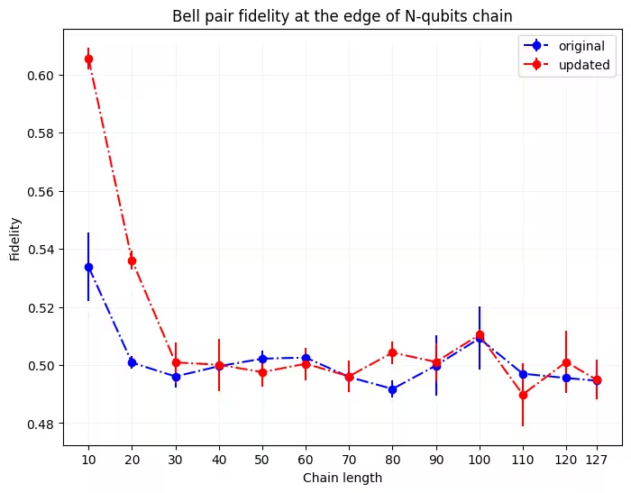
실시간 특성화로 인해 모든 실행에서 성능 향상이 나타나는 것은 아닙니다. 체인 길이가 길어질수록 물리적 Qubit을 선택할 자유도가 줄어들기 때문에 업데이트된 장치 정보의 중요성이 상대적으로 낮아집니다. 하지만 장치 성능을 파악하기 위해 최신 데이터를 수집하는 것은 좋은 관행입니다. 경우에 따라 과도적인 이준위 시스템(transient two-level system)이 일부 Qubit의 성능에 영향을 미칠 수 있습니다. 실시간 데이터를 통해 이러한 이벤트가 발생하는 시점을 파악하고, 그런 상황에서의 실험 실패를 방지할 수 있습니다.
이 방법을 실제 실행에 적용하여 얼마나 많은 이점을 얻을 수 있는지 확인해 보세요! 또한 다양한 Backend에서 얼마나 많은 성능 향상을 얻을 수 있는지도 시험해 보세요.
튜토리얼 설문
이 튜토리얼에 대한 피드백을 제공하기 위해 간단한 설문 조사에 참여해 주세요. 여러분의 의견은 콘텐츠 개선과 사용자 경험 향상에 도움이 됩니다.
Note: This survey is provided by IBM Quantum and relates to the original English content. To give feedback on doQumentation's website, translations, or code execution, please open a GitHub issue.