TEM 함수로 kicked Ising 모델 시뮬레이션

Algorithmiq의 Tensor-network Error Mitigation (TEM) 방법은 고전적 후처리 단계에서 완전히 노이즈 완화를 수행하도록 설계된 하이브리드 양자-고전 알고리즘입니다. TEM을 사용하면 양자 하드웨어에서 불가피하게 발생하는 노이즈로 인한 오류를 완화하면서 더 높은 정확도와 비용 효율성으로 관측량의 기댓값을 계산할 수 있어, 양자 연구자와 산업 실무자 모두에게 매력적인 선택지가 됩니다.

이 튜토리얼은 TEM이 오류 완화 없이는 접근할 수 없고, PEC 및 ZNE와 같은 다른 오류 완화 방법을 사용할 경우 훨씬 더 많은 양자 리소스가 필요한 양자 시스템의 동역학에서 의미 있는 결과를 얻을 수 있음을 보여줍니다.

사용량 추정: 이 노트북은 Heron r3 장치에서 약 10 QPU 분을 사용합니다. 런타임은 선택한 장치에 따라 크게 달라질 수 있습니다. 섹션별 사용량 추정치는 아래에 나와 있습니다.

TEM 함수로 오류 완화된 다체 물리 실험 실행

이 튜토리얼은 다음 참고 문헌을 기반으로 합니다: L. E. Fischer et al., Nat. Phys. (2026). 이 참고 문헌은 최대 91개의 큐비트로 구성된 실제 양자 하드웨어 시뮬레이션을 다룹니다. 이 튜토리얼에서는 더 작은 회로 크기로 유사한 시뮬레이션을 재현합니다.

Kicked Ising 모델은 일반적인 Ising 모델에 해당합니다:

$\hat{H}_{\text{I}} = J \sum_{n=0}^{N-2} \hat{Z}_n \hat{Z}_{n+1} + h \sum_{n=0}^{N-1} \hat{Z}_n$

여기에 횡방향 kick이 적용됩니다:

$\hat{H}_{K} = b \sum_{n=0}^{N-1} \hat{X}_n$

목표는 Floquet 유니타리 $\hat{U}_{\text{KI}} = e^{-i \hat{H}_K} e^{-i \hat{H}_I}$ 로 구현할 수 있는 횡방향 kicked Ising 해밀토니안 하에서의 상태 동역학을 시뮬레이션하는 것입니다. 진화시킬 초기 상태는 첫 번째 큐비트가 $|+\rangle$ 상태에 있고 나머지 큐비트는 쌍을 이루어 Bell 상태 $(|00\rangle + |11\rangle)/\sqrt{2}$ 로 설정된 상태입니다.

관측하려는 양은 상관 함수입니다. 참고 논문에서는 이 양이 $n^{th}$ 큐비트의 $\hat{X}$ Pauli 연산자로 다시 쓸 수 있음을 설명합니다. 여러 물리적 시간 단계 $t$ 후에 Pauli 연산자 $\hat{X}_{n=t}$ 의 값을 계산합니다. 시스템의 파라미터에 따라 이 관측량의 값은 정확하게 계산하거나 근사적인 방법으로만 시뮬레이션할 수 있습니다. 구체적으로 $|J|=|b|=\pi/4$ 일 때 $[\cos(2h)]^t$ 와 같으며, 이는 이 튜토리얼의 결과를 벤치마킹하는 데 사용할 값입니다. 또한 주어진 시간 단계 $t$ 에서 $\langle\hat{X}_{n\neq t}\rangle$ 는 0입니다. 이 값들을 얻는 자세한 방법과 이러한 파라미터 외부의 근사 고전 시뮬레이션 결과와의 비교는 L. E. Fischer et al., Nat. Phys. (2026)을 참조하세요.

TEM은 먼저 회로 내 2큐비트 게이트의 각 고유한 레이어에 대한 노이즈를 특성화하고 판독 오류를 특성화합니다. 그런 다음 양자 기계에서 회로를 실행합니다. 마지막으로 IBM Cloud®의 고전적 리소스에서 텐서 네트워크 오류 완화가 수행되고 완화된 값이 반환됩니다. 이 예에서 회로에는 특성화할 두 개의 고유한 레이어가 있습니다.

설정

전제 조건으로 필요한 종속성이 설치되어 있는지 확인하세요.

%pip install numpy matplotlib qiskit qiskit-ibm-catalog qiskit-ibm-runtime pylatexenc qiskit_qasm3_import

import os
from matplotlib import pyplot as plt
import numpy as np

from qiskit.quantum_info import SparsePauliOp
from qiskit.qasm3 import load

from qiskit_ibm_catalog import QiskitFunctionsCatalog

TEM을 사용한 오류 완화

kicked Ising 모델을 구현하는 회로를 제공합니다. 회로는 다음과 같이 준비됩니다. 첫 번째는 상태 준비 단계로, 첫 번째 큐비트는 $|+\rangle$ 상태에 있고 나머지는 Bell 쌍 $(|00\rangle + |11\rangle)/\sqrt{2}$ 으로 짝을 이룹니다. 이어서 유니타리 $\hat{U}_{\text{KI}}$ 를 구현하는 브릭워크 구조가 옵니다. 물리적 시간 단계의 수는 $t/2$ 회로 레이어에 해당합니다. 다음 코드는 이 튜토리얼에 필요한 두 개의 QASM 파일을 다운로드합니다.

# Download required QASM files
import urllib

urllib.request.urlretrieve(
    "https://ibm.box.com/shared/static/swy5jtq309b0xpzluzlmsmj908yphes8.qasm",
    "ki_30q.qasm",
)
urllib.request.urlretrieve(
    "https://ibm.box.com/shared/static/et3gkodonw6gsp2trs43lzaozrdtiu7s.qasm",
    "ki_12q.qasm",
)

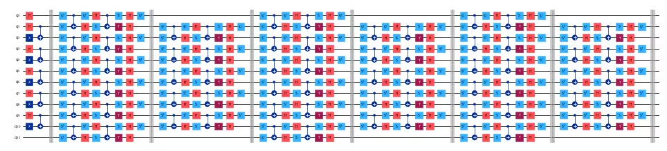
12개의 큐비트와 6개의 시간 단계를 가진 소규모 회로를 시각화할 수 있습니다:

# Parameters of the kicked Ising model
h = 0.0
num_qubits = 12
t_steps = 6

# Load the circuit for the kicked Ising model
small_circuit = load("ki_12q.qasm")

# Draw the circuit
small_circuit.draw("mpl", scale=0.25, fold=-1)

Output of the previous code cell

다음으로 관측량 $\hat{X}_{n=t}$ 를 구성합니다. Qiskit에서 사용하는 순서와 일치하도록 간단한 Pauli 문자열로 구성됩니다:

def xt_observable(n_qubits, t_steps):
    pauli_str = "".join(["I" * t_steps, "X", "I" * (n_qubits - t_steps - 1)])
    pauli_str = pauli_str[::-1]  # Reverse the string to match qiskit order
    return SparsePauliOp(data=pauli_str, coeffs=1.0)

12큐비트 소규모 예시에서 관측량은 다음과 같습니다:

# Build the observable for the kicked Ising model
small_observable = xt_observable(n_qubits=12, t_steps=6)
print(small_observable)

SparsePauliOp(['IIIIIXIIIIII'],
              coeffs=[1.+0.j])

Qiskit Functions는 PUB를 입력을 수집하는 방법으로 사용합니다. 이 경우 단일 회로와 관측량을 PUB로 고려해 봅시다:

# Collect the input PUBs, in this case composed of a
# single circuit and observable
pubs = [(small_circuit, [small_observable])]

다음으로 TEM 함수에 액세스합니다. 먼저 IBM Cloud에 대한 필요한 인증을 설정하고 사용 가능한 장치에서 백엔드를 선택합니다. 토큰, 사용 가능한 백엔드 및 해당 클라우드 리소스 이름(CRN)은 IBM Quantum Platform 대시보드에서 계정에 로그인하여 얻을 수 있습니다.

# Set IBM Quantum credentials and backend configuration
personal_token = os.environ.get(
    "QISKIT_IBM_TOKEN", "<API-KEY>"
)  # Replace with your personal token or set the environment variable
channel = "ibm_quantum_platform"
crn = "your_crn"  # Replace with the Cloud Resource Name (CRN)

# Select the QPU backend
backend_name = "ibm_qpu_name"  # Replace with your desired backend's name

Qiskit Functions Catalog에서 TEM 함수를 로드합니다:

# Load the TEM function from the Qiskit Functions Catalog
catalog = QiskitFunctionsCatalog(
    channel=channel,
    token=personal_token,
    instance=crn,
)
tem = catalog.load("algorithmiq/tem")

TEM이 제공하는 오류 완화로 kicked Ising 회로에서 실험을 실행할 수 있습니다. 기본 설정을 사용하면 QPU에 따라 약 2.5분의 QPU 런타임을 예상하여 간단하게 TEM을 실행할 수 있습니다:

tem_job = tem.run(pubs=pubs, backend_name=backend_name)

기본 옵션을 사용하면 TEM 함수는 양자 컴퓨터에서 세 가지 작업을 실행합니다: 노이즈 학습, 판독 완화, 회로 샘플링. 이 각각에서 사용되는 shots 수는 함수에 전달되는 옵션에서 변경할 수 있습니다. 기본적으로 이 파라미터는 완화된 기댓값에서 0.05의 정밀도를 달성하도록 설정되어 있습니다. 작업 상태는 IBM Quantum Platform 대시보드에서 확인하거나 다음으로 확인할 수 있습니다:

print(tem_job.status())

QUEUED

상태가 DONE이 되면 원시 결과와 완화된 결과를 확인할 수 있습니다. 아래에 정의된 tem_evs는 요청된 관측량의 기댓값(이 경우 단 하나의 관측량 $\langle \hat X_{n=t}\rangle$ )이고, tem_std는 해당 표준 편차입니다.

# Get the results of the TEM job
tem_results = tem_job.result()[
    0
]  # Get the first and only result from the job
tem_evs = tem_results.data.evs[0]
tem_std = tem_results.data.stds[0]

print(f"TEM Result: {tem_evs:.3f} ± {tem_std:.3f}")

TEM Result: 1.031 ± 0.046

또한 IBM Quantum Platform에서 각 호출에 사용된 양자 런타임을 확인하거나 Python 코드에서 결과 메타데이터를 검사할 수도 있습니다.

# Get the TEM job runtime
tem_runtime = tem_job.result().metadata["resource_usage"][
    "RUNNING: EXECUTING_QPU"
]["QPU_TIME"]

print(f"TEM Runtime: {tem_runtime} seconds")

TEM Runtime: 155.0 seconds

TEM 파라미터 및 고급 옵션 사용자 정의

TEM 함수는 오류 완화 워크플로를 사용자 정의할 수 있는 여러 고급 옵션을 제공합니다. 이러한 옵션을 통해 정밀도, shots 수, 노이즈 학습 전략 및 기타 파라미터를 제어하여 실험의 요구 사항과 사용 가능한 양자 리소스에 더 잘 맞출 수 있습니다.

일반적인 고급 옵션은 다음과 같습니다:

precision: 완화된 기댓값의 목표 정밀도를 지정합니다.
default_shots: precision 대신 측정 작업에서 사용되는 shots 수를 지정할 수 있습니다.
tem_max_bond_dimension: 텐서 네트워크에서 사용되는 최대 본드 차원.
tem_compression_cutoff: 텐서 네트워크에 사용할 컷오프 값.
노이즈 학습 옵션: 반복 횟수나 특정 보정 회로 등 노이즈를 어떻게 특성화할지 구성합니다.
private: 회로와 실험 결과를 비공개로 유지하고 작업 결과의 여러 번 다운로드를 비활성화합니다.

지원되는 옵션의 전체 목록과 설명은 TEM 문서 또는 Qiskit Functions Catalog를 참조하세요. 이러한 파라미터를 조정하여 런타임, 리소스 사용량, 결과 정확도 간의 균형을 맞출 수 있습니다. TEM 함수를 실행할 때 이러한 옵션을 딕셔너리로 options 인수에 전달할 수 있습니다:

options = {
    "default_shots": 10_000,
    "tem_max_bond_dimension": 512,
    "tem_compression_cutoff": 1e-16,
    # This option helps optimizing the measurement
    # stage since the observable is strongly biased
    # toward the X operator for all the qubits.
    "compute_shadows_bias_from_observable": True,
    # set to True to keep experiment results private,
    # recommended for confidential circuits
    "private": False,
}

노이즈 학습기에 대한 사용자 정의 옵션도 전달할 수 있습니다. 이는 Qiskit Runtime NoiseLearnerOptions에서 사용되는 정의를 따릅니다:

nl_options = {
    "num_randomizations": 32,
    "max_layers_to_learn": 2,
    "shots_per_randomization": 128,
    "layer_pair_depths": [0, 1, 2, 4, 16, 32],
}

# add noise learning options to the overall options
options |= nl_options

회로에 맞게 조정된 이러한 사용자 정의 옵션으로 실험을 다시 실행합니다. 예상 런타임은 약 4 QPU 분입니다.

tem_job_custom = tem.run(
    pubs=pubs, backend_name=backend_name, options=options
)

작업이 비공개로 설정되지 않은 경우 나중에 결과를 복구할 수 있습니다. 그러려면 여기에 출력된 작업 ID를 저장하고 tem_job_custom = catalog.get_job_by_id("your-job-id")를 사용하세요.

job_id = tem_job_custom.job_id
print(f"Job ID: {job_id}")

Job ID: 1ba10094-a541-457a-9287-dbd49306d12d

results_custom = tem_job_custom.result()
tem_evs = results_custom[0].data.evs[0]
tem_std = results_custom[0].data.stds[0]

print(f"TEM Result: {tem_evs:.3f} ± {tem_std:.3f}")

TEM Result: 0.956 ± 0.018

이제 결과와 메타데이터를 검사하여 실험에 대한 통찰을 얻을 수 있습니다:

metadata_custom = results_custom[0].metadata

unmitigated_evs = metadata_custom["evs_non_mitigated"][0]
unmitigated_stds = metadata_custom["stds_non_mitigated"][0]
print(f"Unmitigated Result: {unmitigated_evs:.3f} ± {unmitigated_stds:.3f}")

# Exact result for the kicked Ising model from the reference paper
exact_evs = np.cos(2 * h) ** t_steps
print("Exact Result:", exact_evs)

Unmitigated Result: 0.894 ± 0.015
Exact Result: 1.0

# Plot comparing the different expectation values
plt.bar(
    ["Unmitigated", "TEM"],
    [unmitigated_evs, tem_evs],
    yerr=[unmitigated_stds, tem_std],
    color=["grey", "c"],
)
plt.hlines(y=exact_evs, xmin=-0.5, xmax=1.5, colors="r", linestyles="dashed")
plt.ylabel("Expectation Value")
plt.ylim(0, 1.1)
plt.show()

Output of the previous code cell

마지막으로 사용자 정의 옵션이 QPU 및 고전적 런타임에 미치는 영향을 확인할 수 있습니다:

# Get the metadata of the TEM job
job_metadata = results_custom.metadata

# Get the runtime of the TEM job
qpu_runtime = job_metadata["resource_usage"]["RUNNING: EXECUTING_QPU"][
    "QPU_TIME"
]
classical_runtime = (
    job_metadata["resource_usage"]["RUNNING: OPTIMIZING_FOR_HARDWARE"][
        "CPU_TIME"
    ]
    + job_metadata["resource_usage"]["RUNNING: POST_PROCESSING"]["CPU_TIME"]
)

print(f"QPU Runtime: {qpu_runtime} seconds")
print(f"Classical Runtime: {classical_runtime} seconds")

QPU Runtime: 342.0 seconds
Classical Runtime: 107.632604 seconds

대규모 회로로 TEM 확장

대규모 회로는 원칙적으로 TEM 함수로 실행할 수 있습니다. 그러나 TEM은 IBM Cloud 러너에서 실행되므로 잠재적으로 매우 긴 실행 시간이 발생할 수 있어 고전적 리소스의 한계를 인식하는 것이 중요합니다. 매우 큰 회로의 경우 qiskit_ibm@algorithmiq.fi의 TEM 지원 팀에 문의하세요.

여기서는 더 큰 유틸리티 규모의 30큐비트 회로 예제를 실행하며 정확도보다 속도에 맞게 TEM 파라미터를 최적화합니다.

# Kicked Ising model parameters
n_qubits = 30
t_steps = 15
h = 0.0

# Load the circuit for the kicked Ising model
circuit = load("ki_30q.qasm")

# Build the observable for the kicked Ising model
observable = xt_observable(n_qubits=n_qubits, t_steps=t_steps)

# Collect the input PUBs, in this case composed of a
# single circuit and observable
pubs = [(circuit, [observable])]

성능 지향 옵션을 정의해 봅시다:

options = {
    "num_randomizations": 32,
    "max_layers_to_learn": 2,
    "shots_per_randomization": 128,
    "layer_pair_depths": [0, 1, 2, 4, 16, 32, 64],
    "default_shots": 5_000,
    "tem_max_bond_dimension": 128,
    "tem_compression_cutoff": 1e-10,
    "compute_shadows_bias_from_observable": True,
    "private": False,
}

마지막으로 실험을 실행하고 결과를 얻어 시각화합니다. 이 과정은 약 3.5 QPU 분이 걸립니다.

tem_job_large = tem.run(pubs=pubs, backend_name=backend_name, options=options)

job_id = tem_job_large.job_id
print(f"Job ID: {job_id}")

Job ID: 9f3f190f-f4b0-4dcb-bb83-5f71f37d0d77

results_large = tem_job_large.result()
tem_evs = results_large[0].data.evs[0]
tem_std = results_large[0].data.stds[0]

print(f"TEM Result: {tem_evs:.3f} ± {tem_std:.3f}")

# Get the metadata of the TEM job
job_metadata = tem_job_large.result().metadata

# Get the runtime of the TEM job
qpu_runtime = job_metadata["resource_usage"]["RUNNING: EXECUTING_QPU"][
    "QPU_TIME"
]
classical_runtime = (
    job_metadata["resource_usage"]["RUNNING: OPTIMIZING_FOR_HARDWARE"][
        "CPU_TIME"
    ]
    + job_metadata["resource_usage"]["RUNNING: POST_PROCESSING"]["CPU_TIME"]
)

print(f"QPU Runtime: {qpu_runtime} seconds")
print(f"Classical Runtime: {classical_runtime} seconds")

TEM Result: 0.794 ± 0.026
QPU Runtime: 203.0 seconds
Classical Runtime: 251.71805499999996 seconds

# Plot comparing the different expectation values
metadata_large = results_large[0].metadata
unmitigated_evs = metadata_large["evs_non_mitigated"][0]
unmitigated_stds = metadata_large["stds_non_mitigated"][0]

exact_evs = np.cos(2 * h) ** t_steps

plt.bar(
    ["Unmitigated", "TEM"],
    [unmitigated_evs, tem_evs],
    yerr=[unmitigated_stds, tem_std],
    color=["grey", "c"],
)
plt.hlines(y=exact_evs, xmin=-0.5, xmax=1.5, colors="r", linestyles="dashed")
plt.ylabel("Expectation Value")
plt.ylim(0, 1.1)
plt.show()

Output of the previous code cell

TEM 함수로 오류 완화된 다체 물리 실험 실행​

설정​

TEM을 사용한 오류 완화​

TEM 파라미터 및 고급 옵션 사용자 정의​

대규모 회로로 TEM 확장​

TEM 함수로 오류 완화된 다체 물리 실험 실행

설정

TEM을 사용한 오류 완화

TEM 파라미터 및 고급 옵션 사용자 정의

대규모 회로로 TEM 확장