예제 및 응용

이 강의에서는 몇 가지 변분 알고리즘 예제와 그 적용 방법을 살펴봅니다:

• 사용자 정의 변분 알고리즘 작성 방법
• 변분 알고리즘을 활용해 최솟값 고유값을 구하는 방법
• 변분 알고리즘을 응용 사례에 적용하는 방법

여기서 소개하는 모든 문제에 Qiskit 패턴 프레임워크를 적용할 수 있습니다. 그러나 반복을 줄이기 위해, 실제 하드웨어에서 실행하는 하나의 예제 사례에서만 프레임워크 단계를 명시적으로 설명합니다.

문제 정의

다음 관측량의 고유값을 변분 알고리즘으로 구하고자 한다고 가정해 봅시다:

$$\hat{O}_1 = 2 II - 2 XX + 3 YY - 3 ZZ,$$

이 관측량의 고유값은 다음과 같습니다:

$$\left\{ \begin{array}{c} \lambda_0 = -6 \\ \lambda_1 = 4 \\ \lambda_2 = 4 \\ \lambda_3 = 6 \end{array} \right\}$$

그리고 고유 상태는 다음과 같습니다:

$$\left\{ \begin{array}{c} |\phi_0\rangle = \frac{1}{\sqrt{2}}(|00\rangle + |11\rangle)\\ |\phi_1\rangle = \frac{1}{\sqrt{2}}(|00\rangle - |11\rangle)\\ |\phi_2\rangle = \frac{1}{\sqrt{2}}(|01\rangle - |10\rangle)\\ |\phi_3\rangle = \frac{1}{\sqrt{2}}(|01\rangle + |10\rangle) \end{array} \right\}$$

# Added by doQumentation — required packages for this notebook
!pip install -q numpy qiskit qiskit-ibm-runtime rustworkx scipy

from qiskit.quantum_info import SparsePauliOp

observable_1 = SparsePauliOp.from_list([("II", 2), ("XX", -2), ("YY", 3), ("ZZ", -3)])

사용자 정의 VQE

먼저 $\hat{O}_1$의 최솟값 고유값을 구하기 위해 VQE 인스턴스를 직접 구성하는 방법을 살펴봅니다. 이 과정에서 이 과정 전반에 걸쳐 다룬 다양한 기법들을 활용합니다.

def cost_func_vqe(params, ansatz, hamiltonian, estimator):
    """Return estimate of energy from estimator

    Parameters:
        params (ndarray): Array of ansatz parameters
        ansatz (QuantumCircuit): Parameterized ansatz circuit
        hamiltonian (SparsePauliOp): Operator representation of Hamiltonian
        estimator (Estimator): Estimator primitive instance

    Returns:
        float: Energy estimate
    """
    pub = (ansatz, hamiltonian, params)
    cost = estimator.run([pub]).result()[0].data.evs

    return cost

from qiskit.circuit.library.n_local import n_local
from qiskit import QuantumCircuit

import numpy as np

reference_circuit = QuantumCircuit(2)
reference_circuit.x(0)

variational_form = n_local(
    num_qubits=2,
    rotation_blocks=["rz", "ry"],
    entanglement_blocks="cx",
    entanglement="linear",
    reps=1,
)

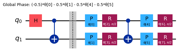
raw_ansatz = reference_circuit.compose(variational_form)
raw_ansatz.decompose().draw("mpl")

먼저 로컬 시뮬레이터에서 디버깅을 시작합니다.

from qiskit.primitives import StatevectorEstimator as Estimator
from qiskit.primitives import StatevectorSampler as Sampler

estimator = Estimator()
sampler = Sampler()

이제 초기 파라미터 세트를 설정합니다:

x0 = np.ones(raw_ansatz.num_parameters)
print(x0)

[1. 1. 1. 1. 1. 1. 1. 1.]

이 비용 함수를 최소화하여 최적 파라미터를 계산할 수 있습니다.

# SciPy minimizer routine
from scipy.optimize import minimize
import time

start_time = time.time()

result = minimize(
    cost_func_vqe,
    x0,
    args=(raw_ansatz, observable_1, estimator),
    method="COBYLA",
    options={"maxiter": 1000, "disp": True},
)

end_time = time.time()
execution_time = end_time - start_time

Return from COBYLA because the trust region radius reaches its lower bound.
Number of function values = 103   Least value of F = -5.999999998357189
The corresponding X is:
[2.27483579e+00 8.37593091e-01 1.57080508e+00 5.82932911e-06
 2.49973063e+00 6.41884255e-01 6.33686904e-01 6.33688223e-01]

result

message: Return from COBYLA because the trust region radius reaches its lower bound.
 success: True
  status: 0
     fun: -5.999999998357189
       x: [ 2.275e+00  8.376e-01  1.571e+00  5.829e-06  2.500e+00
            6.419e-01  6.337e-01  6.337e-01]
    nfev: 103
   maxcv: 0.0

이 예제는 Qubit이 두 개뿐이므로, NumPy의 선형 대수 고유값 솔버를 사용해 결과를 검증할 수 있습니다.

from numpy.linalg import eigvalsh

solution_eigenvalue = min(eigvalsh(observable_1.to_matrix()))

print(f"""Number of iterations: {result.nfev}""")
print(f"""Time (s): {execution_time}""")

print(
    f"Percent error: {100*abs((result.fun - solution_eigenvalue)/solution_eigenvalue):.2e}"
)

Number of iterations: 103
Time (s): 0.4394676685333252
Percent error: 2.74e-08

보면 알 수 있듯이, 결과가 이상적인 값에 매우 가깝습니다.

속도와 정확도 향상을 위한 실험

기준 상태 추가

앞선 예제에서는 기준 연산자 $U_R$을 사용하지 않았습니다. 이제 이상적인 고유 상태 $\frac{1}{\sqrt{2}}(|00\rangle + |11\rangle)$를 어떻게 얻을 수 있는지 생각해 보겠습니다. 다음 Circuit을 살펴보세요.

from qiskit import QuantumCircuit

ideal_qc = QuantumCircuit(2)
ideal_qc.h(0)
ideal_qc.cx(0, 1)

ideal_qc.draw("mpl")

이 Circuit이 원하는 상태를 만들어 내는지 빠르게 확인할 수 있습니다.

from qiskit.quantum_info import Statevector

Statevector(ideal_qc)

Statevector([0.70710678+0.j, 0.        +0.j, 0.        +0.j,
             0.70710678+0.j],
            dims=(2, 2))

해 상태를 준비하는 Circuit이 어떻게 생겼는지 확인했으므로, Hadamard Gate를 기준 Circuit으로 사용하는 것이 합리적입니다. 이렇게 하면 전체 ansatz는 다음과 같이 구성됩니다.

reference = QuantumCircuit(2)
reference.h(0)
reference.cx(0, 1)
# Include barrier to separate reference from variational form
reference.barrier()

ref_ansatz = variational_form.decompose().compose(reference, front=True)

ref_ansatz.draw("mpl")

이 새로운 Circuit에서는 모든 파라미터를 $0$으로 설정했을 때 이상적인 해에 도달할 수 있으므로, 기준 Circuit 선택이 합리적임을 확인할 수 있습니다.

이제 이전 시도와 비교하여 비용 함수 평가 횟수, 최적화 반복 횟수, 소요 시간을 비교해 보겠습니다.

import time

start_time = time.time()

ref_result = minimize(
    cost_func_vqe, x0, args=(ref_ansatz, observable_1, estimator), method="COBYLA"
)

end_time = time.time()
execution_time = end_time - start_time

최적 파라미터를 사용하여 최솟값 고유값을 계산합니다.

experimental_min_eigenvalue_ref = cost_func_vqe(
    ref_result.x, ref_ansatz, observable_1, estimator
)
print(experimental_min_eigenvalue_ref)

-5.999999996759607

print("ADDED REFERENCE STATE:")
print(f"""Number of iterations: {ref_result.nfev}""")
print(f"""Time (s): {execution_time}""")
print(
    f"Percent error: {100*abs((experimental_min_eigenvalue_ref - solution_eigenvalue)/solution_eigenvalue):.2e}"
)

ADDED REFERENCE STATE:
Number of iterations: 127
Time (s): 0.5620882511138916
Percent error: 5.40e-08

시스템 환경에 따라, 이 매우 소규모 예제에서는 속도나 정확도가 개선될 수도 있고 그렇지 않을 수도 있습니다. 중요한 점은 물리적으로 동기 부여된 기준 상태로 시작하는 것이, 문제의 규모가 커질수록 속도와 정확도를 높이는 데 점점 더 중요해진다는 것입니다.

초기점 변경

기준 상태 추가의 효과를 살펴보았으니, 이제 서로 다른 초기점 $\vec{\theta_0}$을 선택했을 때 어떤 일이 일어나는지 알아보겠습니다. 특히 $\vec{\theta_0}=(0,0,0,0,6,0,0,0)$과 $\vec{\theta_0}=(6,6,6,6,6,6,6,6,6)$를 사용해 보겠습니다.

기준 상태를 도입할 때 논의했듯이, 모든 파라미터가 $0$일 때 이상적인 해가 얻어지므로 첫 번째 초기점에서 더 적은 평가 횟수가 소요될 것입니다.

import time

start_time = time.time()

x0 = [0, 0, 0, 0, 6, 0, 0, 0]

x0_1_result = minimize(
    cost_func_vqe, x0, args=(raw_ansatz, observable_1, estimator), method="COBYLA"
)

end_time = time.time()
execution_time = end_time - start_time

print("INITIAL POINT 1:")
print(f"""Number of iterations: {x0_1_result.nfev}""")
print(f"""Time (s): {execution_time}""")

INITIAL POINT 1:
Number of iterations: 108
Time (s): 0.4492197036743164

초기점을 $\vec{\theta_0}=(6,6,6,6,6,6,6,6,6)$로 조정합니다.

import time

start_time = time.time()

x0 = 6 * np.ones(raw_ansatz.num_parameters)

x0_2_result = minimize(
    cost_func_vqe, x0, args=(raw_ansatz, observable_1, estimator), method="COBYLA"
)

end_time = time.time()
execution_time = end_time - start_time

print("INITIAL POINT 2:")
print(f"""Number of iterations: {x0_2_result.nfev}""")
print(f"""Time (s): {execution_time}""")

INITIAL POINT 2:
Number of iterations: 107
Time (s): 0.40889453887939453

다양한 초기점을 실험해 보면 더 적은 함수 평가 횟수로 더 빠르게 수렴할 수도 있습니다.

다양한 최적화기 실험

SciPy minimize의 method 인수를 통해 최적화기를 변경할 수 있으며, 더 많은 옵션은 여기에서 확인할 수 있습니다. 앞서는 제약 있는 최솟값 탐색기(COBYLA)를 사용했습니다. 이번 예제에서는 제약 없는 최솟값 탐색기(BFGS)를 사용해 보겠습니다.

import time

start_time = time.time()

result = minimize(
    cost_func_vqe, x0, args=(raw_ansatz, observable_1, estimator), method="BFGS"
)

end_time = time.time()
execution_time = end_time - start_time

print("CHANGED TO BFGS OPTIMIZER:")
print(f"""Number of iterations: {result.nfev}""")
print(f"""Time (s): {execution_time}""")

CHANGED TO BFGS OPTIMIZER:
Number of iterations: 117
Time (s): 0.31656408309936523

VQD 예제

여기서는 Qiskit 패턴 프레임워크를 명시적으로 구현합니다.

1단계: 고전적 입력을 양자 문제로 매핑하기

이제 관측 가능량의 가장 낮은 고유값만 찾는 것이 아니라, 모든 $4$개의 고유값을 찾겠습니다 ($k=4$).

VQD의 비용 함수는 다음과 같다는 점을 기억하세요:

$$C_{l}(\vec{\theta}) := \langle \psi(\vec{\theta}) | \hat{H} | \psi(\vec{\theta})\rangle + \sum_{j=0}^{l-1}\beta_j |\langle \psi(\vec{\theta})| \psi(\vec{\theta^j})\rangle |^2 \quad \forall l\in\{1,\cdots,k\}=\{1,\cdots,4\}$$

이 점이 특히 중요한 이유는, VQD 객체를 정의할 때 벡터 $\vec{\beta}=(\beta_0,\cdots,\beta_{k-1})$ (이 경우에는 $(\beta_0, \beta_1, \beta_2, \beta_3)$)를 인수로 전달해야 하기 때문입니다.

또한 Qiskit의 VQD 구현에서는, 이전 노트북에서 설명한 유효 관측 가능량을 고려하는 대신, 충실도(fidelity) $|\langle \psi(\vec{\theta})| \psi(\vec{\theta^j})\rangle |^2$를 ComputeUncompute 알고리즘을 통해 직접 계산합니다. 이 알고리즘은 Sampler 프리미티브를 활용하여 회로 $U_A^\dagger(\vec{\theta})U_A(\vec{\theta^j})$에서 $|0\rangle$을 얻을 확률을 샘플링합니다. 이 확률이 정확히

$$\begin{aligned} p_0 & = |\langle 0|U_A^\dagger(\vec{\theta})U_A(\vec{\theta^j})|0\rangle|^2 \\[1mm] & = |\big(\langle 0|U_A^\dagger(\vec{\theta})\big)\big(U_A(\vec{\theta^j})|0\rangle\big)|^2 \\[1mm] & = |\langle \psi(\vec{\theta}) |\psi(\vec{\theta^j}) \rangle|^2 \\[1mm] \end{aligned}$$

이기 때문에 이 방법이 성립합니다.

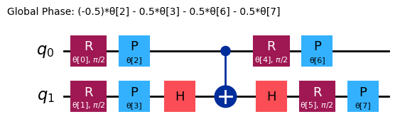
ansatz = n_local(
    num_qubits=2,
    rotation_blocks=["ry", "rz"],
    entanglement_blocks="cz",
    #    entanglement="linear",
    reps=1,
)

ansatz.decompose().draw("mpl")

다음 관측 가능량을 살펴보겠습니다:

$$\hat{O}_2 := 2 II - 3 XX + 2 YY - 4 ZZ$$

이 관측 가능량의 고유값은 다음과 같습니다:

$$\left\{ \begin{array}{c} \lambda_0 = -7 \\ \lambda_1 = 3\\ \lambda_2 = 5 \\ \lambda_3 = 7 \end{array} \right\}$$

그리고 고유 상태는 다음과 같습니다:

$$\left\{ \begin{array}{c} |\phi_0\rangle = \frac{1}{\sqrt{2}}(|00\rangle + |11\rangle)\\ |\phi_1\rangle = \frac{1}{\sqrt{2}}(|00\rangle - |11\rangle)\\ |\phi_2\rangle = \frac{1}{\sqrt{2}}(|01\rangle + |10\rangle)\\ |\phi_3\rangle = \frac{1}{\sqrt{2}}(|01\rangle - |10\rangle) \end{array} \right\}$$

from qiskit.quantum_info import SparsePauliOp

observable_2 = SparsePauliOp.from_list([("II", 2), ("XX", -3), ("YY", 2), ("ZZ", -4)])

이제 겹침 페널티(overlap penalty)를 계산하는 함수를 추가합니다. 이 함수는 여전히 문제를 양자 회로에 매핑하는 단계의 일부입니다. 하지만 이전 강의에서 설명한 바와 같이, 이 함수는 현재 변분 회로와 이전에 최적화된 회로(더 낮은 에너지/비용 상태에서 얻은 것) 사이의 겹침을 계산합니다. 새로 생성되는 회로도 실제 하드웨어에서 실행하려면 Transpile이 필요합니다. 이 함수는 이전에 시뮬레이터에서 사용하는 것을 본 적이 있습니다. 여기서는 실제 Backend를 사용할 때의 Transpile 및 관련 최적화를 미리 고려해야 하므로, if realbackend == 1 주변의 코드가 추가되었습니다. 이는 2단계의 내용이 일부 섞인 것이지만, 2단계는 이후에 명시적으로 다루겠습니다.

import numpy as np
from qiskit.transpiler.preset_passmanagers import generate_preset_pass_manager

def calculate_overlaps(
    ansatz, prev_circuits, parameters, sampler, realbackend, backend
):
    def create_fidelity_circuit(circuit_1, circuit_2):
        if len(circuit_1.clbits) > 0:
            circuit_1.remove_final_measurements()
        if len(circuit_2.clbits) > 0:
            circuit_2.remove_final_measurements()

        circuit = circuit_1.compose(circuit_2.inverse())
        circuit.measure_all()
        return circuit

    overlaps = []

    for prev_circuit in prev_circuits:
        fidelity_circuit = create_fidelity_circuit(ansatz, prev_circuit)
        if realbackend == 1:
            pm = generate_preset_pass_manager(backend=backend, optimization_level=3)
            fidelity_circuit = pm.run(fidelity_circuit)
        sampler_job = sampler.run([(fidelity_circuit, parameters)])
        meas_data = sampler_job.result()[0].data.meas

        counts_0 = meas_data.get_int_counts().get(0, 0)
        shots = meas_data.num_shots
        overlap = counts_0 / shots
        overlaps.append(overlap)

    return np.array(overlaps)

이제 VQD의 비용 함수를 추가합니다. 이전 강의와 비교하면, 실제 Backend를 사용할 때 Transpile을 처리하기 위한 두 개의 추가 인수(realbackend와 backend)가 포함되어 있습니다.

def cost_func_vqd(
    parameters,
    ansatz,
    prev_states,
    step,
    betas,
    estimator,
    sampler,
    hamiltonian,
    realbackend,
    backend,
):
    estimator_job = estimator.run([(ansatz, hamiltonian, [parameters])])

    total_cost = 0

    if step > 1:
        overlaps = calculate_overlaps(
            ansatz, prev_states, parameters, sampler, realbackend, backend
        )
        total_cost = np.sum(
            [np.real(betas[state] * overlap) for state, overlap in enumerate(overlaps)]
        )

    estimator_result = estimator_job.result()[0]

    value = estimator_result.data.evs[0] + total_cost

    return value

다시 한번, 디버깅에는 시뮬레이터를 사용한 후 실제 하드웨어로 이동하겠습니다.

from qiskit.primitives import StatevectorSampler
from qiskit.primitives import StatevectorEstimator

sampler = StatevectorSampler(default_shots=4092)
estimator = StatevectorEstimator()

여기서는 계산하고자 하는 상태의 수, 페널티, 그리고 초기 파라미터 집합 x0를 설정합니다.

from qiskit.quantum_info import SparsePauliOp

k = 4
betas = [50, 60, 40]
x0 = np.ones(8)

이제 시뮬레이터를 사용하여 알고리즘을 테스트해 보겠습니다:

from scipy.optimize import minimize

prev_states = []
prev_opt_parameters = []
eigenvalues = []

realbackend = 0

for step in range(1, k + 1):
    if step > 1:
        prev_states.append(ansatz.assign_parameters(prev_opt_parameters))

    result = minimize(
        cost_func_vqd,
        x0,
        args=(
            ansatz,
            prev_states,
            step,
            betas,
            estimator,
            sampler,
            observable_2,
            realbackend,
            None,
        ),
        method="COBYLA",
        options={"maxiter": 200, "tol": 0.000001},
    )
    print(result)

    prev_opt_parameters = result.x
    eigenvalues.append(result.fun)

message: Return from COBYLA because the trust region radius reaches its lower bound.
 success: True
  status: 0
     fun: -6.9999999999996
       x: [ 1.571e+00  1.571e+00  2.519e+00  2.100e+00  1.242e+00
            6.935e-01  2.298e+00  1.991e+00]
    nfev: 151
   maxcv: 0.0
 message: Return from COBYLA because the trust region radius reaches its lower bound.
 success: True
  status: 0
     fun: 3.698974255258432
       x: [ 1.269e+00  1.109e+00  1.080e+00  1.200e+00  1.094e+00
            1.163e+00  9.752e-01  9.519e-01]
    nfev: 103
   maxcv: 0.0
 message: Return from COBYLA because the trust region radius reaches its lower bound.
 success: True
  status: 0
     fun: 4.731320121938101
       x: [ 1.533e+00  2.451e+00  2.526e+00  2.406e+00  1.968e+00
            2.105e+00  8.537e-01  8.442e-01]
    nfev: 110
   maxcv: 0.0
 message: Return from COBYLA because the trust region radius reaches its lower bound.
 success: True
  status: 0
     fun: 7.008239313655201
       x: [ 4.150e+00  2.120e+00  3.495e+00  7.262e-01  1.953e+00
           -1.982e-01  3.263e-01  2.563e+00]
    nfev: 126
   maxcv: 0.0

eigenvalues

[np.float64(-6.9999999999996),
 np.float64(3.698974255258432),
 np.float64(4.731320121938101),
 np.float64(7.008239313655201)]

이 결과는 근사 오차와 전역 위상을 제외하면 예상 결과에 상당히 근접합니다. 고전 최적화기의 허용 오차(tolerance)와 상태 벡터 겹침에 대한 페널티를 조정하면 더 정밀한 값을 얻을 수 있습니다.

solution_eigenvalues = [-7, 3, 5, 7]

for index, experimental_eigenvalue in enumerate(eigenvalues):
    solution_eigenvalue = solution_eigenvalues[index]

    print(
        f"Percent error: {abs((experimental_eigenvalue - solution_eigenvalue)/solution_eigenvalue):.2e}"
    )

Percent error: 5.71e-14
Percent error: 2.33e-01
Percent error: 5.37e-02
Percent error: 1.18e-03

베타 값 변경

이전 레슨에서 언급했듯이, $\vec{\beta}$의 값은 고유값 간의 차이보다 커야 합니다. 조건을 만족하지 않을 때 $\hat{O}_2$에 어떤 일이 발생하는지 살펴보겠습니다.

$$\hat{O}_2 = 2 II - 3 XX + 2 YY - 4 ZZ$$

고유값은 다음과 같습니다.

$$\left\{ \begin{array}{c} \lambda_0 = -7 \\ \lambda_1 = 3\\ \lambda_2 = 5 \\ \lambda_3 = 7 \end{array} \right\}$$

from qiskit.quantum_info import SparsePauliOp

k = 4
betas = np.ones(3)
x0 = np.zeros(8)

from scipy.optimize import minimize

prev_states = []
prev_opt_parameters = []
eigenvalues = []

realbackend = 0

for step in range(1, k + 1):
    if step > 1:
        prev_states.append(ansatz.assign_parameters(prev_opt_parameters))

    result = minimize(
        cost_func_vqd,
        x0,
        args=(
            ansatz,
            prev_states,
            step,
            betas,
            estimator,
            sampler,
            observable_2,
            realbackend,
            None,
        ),
        method="COBYLA",
        options={"tol": 0.01, "maxiter": 200},
    )
    print(result)

    prev_opt_parameters = result.x
    eigenvalues.append(result.fun)

message: Return from COBYLA because the trust region radius reaches its lower bound.
 success: True
  status: 0
     fun: -6.999916534745094
       x: [ 1.568e+00 -1.569e+00  1.385e-01  1.398e-01 -7.972e-01
            7.835e-01 -2.375e-01  4.539e-02]
    nfev: 125
   maxcv: 0.0
 message: Return from COBYLA because the trust region radius reaches its lower bound.
 success: True
  status: 0
     fun: -1.515139929812874
       x: [-5.317e-04 -2.514e-03  1.016e+00  9.998e-01  3.890e-04
            1.772e-04  1.568e-04  8.497e-04]
    nfev: 35
   maxcv: 0.0
 message: Return from COBYLA because the trust region radius reaches its lower bound.
 success: True
  status: 0
     fun: -0.509948114293115
       x: [-3.796e-03  8.853e-03  3.015e-04  9.997e-01  6.271e-04
           -2.554e-03  1.017e-04  2.766e-04]
    nfev: 37
   maxcv: 0.0
 message: Return from COBYLA because the trust region radius reaches its lower bound.
 success: True
  status: 0
     fun: 0.4914672235935682
       x: [-7.178e-03 -8.652e-03  1.125e+00 -5.428e-02 -1.586e-03
            2.031e-03 -3.462e-03  5.734e-03]
    nfev: 35
   maxcv: 0.0

solution_eigenvalues = [-7, 3, 5, 7]

for index, experimental_eigenvalue in enumerate(eigenvalues):
    solution_eigenvalue = solution_eigenvalues[index]

    print(
        f"Percent error: {abs((experimental_eigenvalue - solution_eigenvalue)/solution_eigenvalue):.2e}"
    )

Percent error: 1.19e-05
Percent error: 1.51e+00
Percent error: 1.10e+00
Percent error: 9.30e-01

이번에는 최적화기가 모든 고유 상태에 대해 동일한 상태 $|\phi_0\rangle = \frac{1}{\sqrt{2}}(|00\rangle + |11\rangle)$를 해로 반환합니다. 이는 명백히 잘못된 결과입니다. 베타 값이 너무 작아서 최솟값 고유 상태에 대한 패널티 효과가 충분하지 않았기 때문입니다. 그 결과, 이후 반복에서 해당 상태가 유효 탐색 공간에서 제외되지 않고, 매번 최적 해로 선택되었습니다.

$\vec{\beta}$ 값을 실험적으로 조정하되, 고유값 간의 차이보다 크게 설정할 것을 권장합니다.

2단계: 양자 실행을 위한 문제 최적화

이를 실제 하드웨어에서 실행하려면, 선택한 양자 컴퓨터에 맞게 양자 Circuit을 최적화해야 합니다. 여기서는 가장 유휴 상태인 Backend를 사용하겠습니다.

from qiskit_ibm_runtime import SamplerV2 as Sampler
from qiskit_ibm_runtime import EstimatorV2 as Estimator
from qiskit_ibm_runtime import Session, EstimatorOptions
from qiskit_ibm_runtime import QiskitRuntimeService

service = QiskitRuntimeService()
backend = service.least_busy(operational=True, simulator=False)
# Or use a specific backend
# backend = service.backend("ibm_brisbane")
print(backend)

<IBMBackend('ibm_brisbane')>

사전 설정 패스 매니저와 최적화 수준 3을 사용하여 Circuit을 트랜스파일하겠습니다.

pm = generate_preset_pass_manager(backend=backend, optimization_level=3)
isa_ansatz = pm.run(ansatz)
isa_observable = observable_2.apply_layout(layout=isa_ansatz.layout)

3단계: Qiskit 기본 요소를 사용한 실행

베타 값을 충분히 높게 재설정한 후, 이제 실제 양자 하드웨어에서 계산을 실행할 수 있습니다.

# Estimated compute resource usage: 25 minutes. Benchmarked at 24 min, 30 sec on an Eagle r3 processor on 5-30-24

k = 2
betas = [30, 50, 80]
x0 = np.zeros(8)

real_prev_states = []
real_prev_opt_parameters = []
real_eigenvalues = []

realbackend = 1

estimator_options = EstimatorOptions(resilience_level=1, default_shots=10_000)

with Session(backend=backend) as session:
    estimator = Estimator(mode=session, options=estimator_options)
    sampler = Sampler(mode=session)

    for step in range(1, k + 1):
        if step > 1:
            real_prev_states.append(isa_ansatz.assign_parameters(prev_opt_parameters))

        result = minimize(
            cost_func_vqd,
            x0,
            args=(
                isa_ansatz,
                real_prev_states,
                step,
                betas,
                estimator,
                sampler,
                isa_observable,
                realbackend,
                backend,
            ),
            method="COBYLA",
            options={"maxiter": 200},
        )
        print(result)

        real_prev_opt_parameters = result.x
        real_eigenvalues.append(result.fun)

session.close()
print(real_eigenvalues)

4단계: 후처리 및 고전적 형식으로 결과 반환

출력 결과는 이전 레슨과 예제에서 다루었던 것과 구조적으로 유사합니다. 그러나 위 결과에는 문제가 있는 부분이 있으며, 이를 통해 들뜬 상태(excited states) 맥락에서의 주의 사항을 도출할 수 있습니다. 이 학습 예제에서 사용되는 컴퓨팅 시간을 줄이기 위해, 고전 최적화기의 최대 반복 횟수를 잠재적으로 너무 낮게(200회) 설정했습니다. 앞서 시뮬레이터에서 수행한 계산도 200회 반복 내에서 수렴하지 못했습니다. 이번에는 수렴했지만... 어느 정도의 허용 오차 내에서 수렴한 걸까요? COBYLA가 "수렴 완료"로 판단할 허용 오차를 별도로 지정하지 않았습니다. 함숫값을 보고 이전 실행 결과와 비교해 보면, COBYLA가 우리가 요구하는 정밀도에 근접하지 못했음을 알 수 있습니다.

또 다른 문제도 있습니다. 첫 번째 들뜬 상태의 에너지가 바닥 상태의 에너지보다 낮게 나타납니다! 이것이 어떻게 발생할 수 있는지 생각해 보세요. 힌트: 방금 언급한 수렴 지점과 관련이 있습니다. 이 동작은 VQD를 H2 분자에 적용한 이후에 아래에서 자세히 설명합니다.

양자 화학: 바닥 상태 및 들뜬 상태 에너지 솔버

우리의 목표는 에너지(해밀토니안 $\hat{\mathcal{H}}$)를 나타내는 관측량의 기댓값을 최소화하는 것입니다:

$$\min_{\vec\theta} \langle\psi(\vec\theta)|\hat{\mathcal{H}}|\psi(\vec\theta)\rangle$$

from qiskit.quantum_info import SparsePauliOp
from qiskit.circuit.library import efficient_su2

H2_op = SparsePauliOp.from_list(
    [
        ("II", -1.052373245772859),
        ("IZ", 0.39793742484318045),
        ("ZI", -0.39793742484318045),
        ("ZZ", -0.01128010425623538),
        ("XX", 0.18093119978423156),
    ]
)

chem_ansatz = efficient_su2(H2_op.num_qubits)

chem_ansatz.decompose().draw("mpl")

from qiskit import QuantumCircuit

def cost_func_vqe(params, ansatz, hamiltonian, estimator):
    """Return estimate of energy from estimator

    Parameters:
        params (ndarray): Array of ansatz parameters
        ansatz (QuantumCircuit): Parameterized ansatz circuit
        hamiltonian (SparsePauliOp): Operator representation of Hamiltonian
        estimator (Estimator): Estimator primitive instance

    Returns:
        float: Energy estimate
    """
    pub = (ansatz, hamiltonian, params)
    cost = estimator.run([pub]).result()[0].data.evs
    #    cost = estimator.run(ansatz, hamiltonian, parameter_values=params).result().values[0]
    return cost

이제 초기 파라미터 집합을 설정합니다:

import numpy as np

x0 = np.ones(chem_ansatz.num_parameters)

이 비용 함수를 최소화하여 최적 파라미터를 계산할 수 있으며, 먼저 로컬 시뮬레이터를 사용해 코드를 검증합니다.

from qiskit.primitives import StatevectorEstimator as Estimator
from qiskit.primitives import StatevectorSampler as Sampler

estimator = Estimator()
sampler = Sampler()

# SciPy minimizer routine
from scipy.optimize import minimize
import time

start_time = time.time()

result = minimize(
    cost_func_vqe, x0, args=(chem_ansatz, H2_op, estimator), method="COBYLA"
)

end_time = time.time()
execution_time = end_time - start_time

result

message: Optimization terminated successfully.
 success: True
  status: 1
     fun: -1.857275029048451
       x: [ 7.326e-01  1.354e+00 ...  1.040e+00  1.508e+00]
    nfev: 242
   maxcv: 0.0

비용 함수의 최솟값(-1.857...)은 H2 분자의 바닥 상태 에너지(단위: 하트리)입니다.

들뜬 상태

VQD를 활용하여 총 $k=2$개의 상태(바닥 상태와 첫 번째 들뜬 상태)를 구할 수도 있습니다.

from qiskit.quantum_info import SparsePauliOp
import numpy as np

k = 2
betas = [33, 33]
# x0 = np.zeros(ansatz.num_parameters)
x0 = [
    1.164e00,
    -2.438e-01,
    9.358e-04,
    6.745e-02,
    1.990e00,
    9.810e-02,
    6.154e-01,
    5.454e-01,
]

오버랩 계산을 추가합니다:

from scipy.optimize import minimize

prev_states = []
prev_opt_parameters = []
eigenvalues = []

realbackend = 0

for step in range(1, k + 1):
    if step > 1:
        prev_states.append(ansatz.assign_parameters(prev_opt_parameters))

    result = minimize(
        cost_func_vqd,
        x0,
        args=(
            ansatz,
            prev_states,
            step,
            betas,
            estimator,
            sampler,
            H2_op,
            realbackend,
            None,
        ),
        method="COBYLA",
        options={"tol": 0.001, "maxiter": 2000},
    )
    print(result)

    prev_opt_parameters = result.x
    eigenvalues.append(result.fun)

message: Optimization terminated successfully.
 success: True
  status: 1
     fun: -1.8572671093941977
       x: [ 1.164e+00 -2.437e-01  2.118e-03  6.448e-02  1.990e+00
            9.870e-02  6.167e-01  5.476e-01]
    nfev: 58
   maxcv: 0.0
 message: Optimization terminated successfully.
 success: True
  status: 1
     fun: -1.0322873777662176
       x: [ 3.205e+00  1.502e+00  1.699e+00 -1.107e-02  3.086e+00
            1.530e+00  4.445e-02  7.013e-02]
    nfev: 99
   maxcv: 0.0

eigenvalues

[-1.8572671093941977, -1.0322873777662176]

실제 하드웨어와 최종 주의 사항

이를 실제 하드웨어에서 실행하려면, 사용할 양자 컴퓨터에 맞게 양자 Circuit을 최적화해야 합니다. 여기서는 편의상 가장 한산한 Backend를 사용합니다.

from qiskit_ibm_runtime import SamplerV2 as Sampler
from qiskit_ibm_runtime import EstimatorV2 as Estimator
from qiskit_ibm_runtime import Session, EstimatorOptions
from qiskit_ibm_runtime import QiskitRuntimeService

service = QiskitRuntimeService()
backend = service.least_busy(operational=True, simulator=False)

Transpiler에는 프리셋 패스 매니저를 사용하며, 최적화 수준 3으로 Circuit을 최대한 최적화합니다.

from qiskit.transpiler.preset_passmanagers import generate_preset_pass_manager

pm = generate_preset_pass_manager(backend=backend, optimization_level=3)
isa_ansatz = pm.run(ansatz)
isa_observable = H2_op.apply_layout(layout=isa_ansatz.layout)

VQD는 반복 횟수가 매우 많으므로, 모든 작업을 Runtime Session 내에서 수행합니다. 이렇게 하면 매번 파라미터가 업데이트될 때마다 큐에 추가되는 것이 아니라, 처음 한 번만 큐에 추가됩니다. 비용 함수나 Estimator의 문법은 그 외에 달라지는 부분이 없습니다.

x0 = [
    1.306e00,
    -2.284e-01,
    6.913e-02,
    -2.530e-02,
    1.849e00,
    7.433e-02,
    6.366e-01,
    5.600e-01,
]

# Estimated hardware usage: 20 min benchmarked on an Eagle r3 processor on 5-30-24

real_prev_states = []
real_prev_opt_parameters = []
real_eigenvalues = []

realbackend = 1

estimator_options = EstimatorOptions(resilience_level=1, default_shots=4096)

with Session(backend=backend) as session:
    estimator = Estimator(mode=session)
    sampler = Sampler(mode=session)

    for step in range(1, k + 1):
        if step > 1:
            real_prev_states.append(
                isa_ansatz.assign_parameters(real_prev_opt_parameters)
            )

        result = minimize(
            cost_func_vqd,
            x0,
            args=(
                isa_ansatz,
                real_prev_states,
                step,
                betas,
                estimator,
                sampler,
                isa_observable,
                realbackend,
                backend,
            ),
            method="COBYLA",
            options={"tol": 0.001, "maxiter": 300},
        )
        print(result)

        real_prev_opt_parameters = result.x
        real_eigenvalues.append(result.fun)

session.close()
print(real_eigenvalues)

얻어진 바닥 상태 에너지(-1.83 하트리)는 정확한 값(-1.85 하트리)과 크게 벗어나지 않습니다. 그러나 들뜬 상태 에너지는 상당히 부정확합니다. 이는 이 레슨의 앞부분에서 보았던 오류와 유사한 동작입니다. 들뜬 상태로 보고된 에너지가 바닥 상태의 에너지와 거의 같습니다. 앞선 사례에서는 들뜬 상태 에너지가 보고된 바닥 상태 에너지보다 낮은 값이 나오기도 했습니다.

변분 계산에서는 진정한 바닥 상태 에너지보다 낮은 에너지를 얻는 것이 불가능합니다. 앞선 사례에서 얻은 바닥 상태 에너지가 진정한 바닥 상태에 충분히 가깝지 않았기 때문에 모순이 없었던 것입니다. 이번 경우, 바닥 상태 에너지는 정확한 값에 꽤 근접했음에도 불구하고 들뜬 상태 에너지가 이상하게도 그 값과 거의 같게 나타납니다.

이런 현상이 발생한 이유를 이해하려면, 들뜬 상태를 찾는 방법을 떠올려 보세요. 변분 상태가 바닥 상태와 직교하도록 요구합니다(오버랩 Circuit과 패널티 항을 사용하여). 만약 바닥 상태 에너지를 정확히 구하지 못한 경우(또는 몇 퍼센트 오차가 있는 경우), 정확한 바닥 상태 벡터도 얻지 못하게 됩니다! 따라서 들뜬 상태가 처음 찾은 상태와 직교하도록 요구했을 때, 우리는 진정한 바닥 상태와의 직교성을 부과한 것이 아니라 그 근사값(때로는 형편없는 근사값)과의 직교성을 부과한 것입니다. 그 결과, 들뜬 상태는 진정한 바닥 상태와 직교하도록 강제되지 않았고, 들뜬 상태의 에너지 추정값이 바닥 상태 에너지에 매우 가깝게 나온 것입니다.

이는 VQD에서 항상 주의해야 할 사항입니다. 그러나 원칙적으로, 고전 최적화기의 최대 반복 횟수를 늘리고, 고전 최적화기의 허용 오차를 낮추며, 진정한 바닥 상태를 반복적으로 놓치는 경우 다른 ansatz를 시도하는 방식으로 이를 개선할 수 있습니다. 앞서 살펴본 것처럼 오버랩 패널티(betas)를 수정할 필요도 있을 수 있습니다. 하지만 이는 별개의 문제입니다. 오버랩에 대한 패널티가 아무리 크더라도, 진정한 바닥 상태에 대한 충분히 정확한 추정값을 오버랩 Circuit에서 구하지 못했다면 진정한 바닥 상태를 회피할 수 없습니다.

최적화: Max-Cut

최대 컷(Max-Cut) 문제는 그래프의 꼭짓점을 두 개의 분리된 집합으로 나누어 두 집합 사이의 간선 수를 최대화하는 조합 최적화 문제입니다. 좀 더 형식적으로 설명하면, 꼭짓점 집합 $V$와 간선 집합 $E$로 이루어진 무방향 그래프 $G=(V,E)$가 주어졌을 때, Max-Cut 문제는 꼭짓점을 두 개의 분리된 부분 집합 $S$와 $T$로 분할하여, 한쪽 끝점이 $S$에 있고 다른 쪽 끝점이 $T$에 있는 간선의 수를 최대화하는 것을 목표로 합니다.

Max-Cut은 클러스터링, 네트워크 설계, 상전이 등 다양한 문제에 적용할 수 있습니다. 먼저 문제 그래프를 생성해 보겠습니다.

import rustworkx as rx
from rustworkx.visualization import mpl_draw

n = 4
G = rx.PyGraph()
G.add_nodes_from(range(n))
# The edge syntax is (start, end, weight)
edges = [(0, 1, 1.0), (0, 2, 1.0), (0, 3, 1.0), (1, 2, 1.0), (2, 3, 1.0)]
G.add_edges_from(edges)

mpl_draw(
    G, pos=rx.shell_layout(G), with_labels=True, edge_labels=str, node_color="#1192E8"
)

이 문제는 이진 최적화 문제로 표현할 수 있습니다. 그래프의 꼭짓점 수가 $n$일 때(이 경우 $n=4$), 각 노드 $0 \leq i < n$에 대해 이진 변수 $x_i$를 정의합니다. 이 변수는 노드 $i$가 그룹 $1$에 속하면 $1$, 그룹 $0$에 속하면 $0$의 값을 가집니다. 또한 노드 $i$에서 노드 $j$로 향하는 간선의 가중치를 인접 행렬 $w$의 $(i,j)$ 원소인 $w_{ij}$로 표기합니다. 그래프가 무방향이므로 $w_{ij}=w_{ji}$입니다. 이를 바탕으로 다음 비용 함수를 최대화하는 문제로 표현할 수 있습니다.

$$\begin{aligned} C(\vec{x}) & =\sum_{i,j=0}^n w_{ij} x_i(1-x_j)\\[1mm] & = \sum_{i,j=0}^n w_{ij} x_i - \sum_{i,j=0}^n w_{ij} x_ix_j\\[1mm] & = \sum_{i,j=0}^n w_{ij} x_i - \sum_{i=0}^n \sum_{j=0}^i 2w_{ij} x_ix_j \end{aligned}$$

양자 컴퓨터로 이 문제를 풀기 위해 비용 함수를 관측량의 기댓값으로 표현해야 합니다. 그런데 Qiskit이 기본적으로 지원하는 관측량은 파울리 연산자로 구성되며, 그 고유값이 $0$과 $1$이 아닌 $1$과 $-1$입니다. 따라서 다음과 같은 변수 치환을 수행합니다.

여기서 $\vec{x}=(x_0,x_1,\cdots ,x_{n-1})$입니다. 인접 행렬 $w$를 사용하면 모든 간선의 가중치에 편리하게 접근할 수 있으며, 이를 통해 비용 함수를 도출합니다.

$$z_i = 1-2x_i \rightarrow x_i = \frac{1-z_i}{2}$$

이로부터 다음이 성립합니다.

$$\begin{array}{lcl} x_i=0 & \rightarrow & z_i=1 \\ x_i=1 & \rightarrow & z_i=-1.\end{array}$$

따라서 최대화하고자 하는 새로운 비용 함수는 다음과 같습니다.

$$\begin{aligned} C(\vec{z}) & = \sum_{i,j=0}^n w_{ij} \bigg(\frac{1-z_i}{2}\bigg)\bigg(1-\frac{1-z_j}{2}\bigg)\\[1mm] & = \sum_{i,j=0}^n \frac{w_{ij}}{4} - \sum_{i,j=0}^n \frac{w_{ij}}{4} z_iz_j\\[1mm] & = \sum_{i=0}^n \sum_{j=0}^i \frac{w_{ij}}{2} - \sum_{i=0}^n \sum_{j=0}^i \frac{w_{ij}}{2} z_iz_j \end{aligned}$$

또한 양자 컴퓨터는 최댓값이 아닌 최솟값(보통 가장 낮은 에너지)을 자연스럽게 탐색하므로, $C(\vec{z})$를 최대화하는 대신 다음을 최소화합니다.

$$-C(\vec{z}) = \sum_{i=0}^n \sum_{j=0}^i \frac{w_{ij}}{2} z_iz_j - \sum_{i=0}^n \sum_{j=0}^i \frac{w_{ij}}{2}$$

이제 변수값이 $-1$과 $1$인 최소화할 비용 함수를 갖게 되었으므로, 파울리 $Z$와 다음과 같은 대응 관계를 설정할 수 있습니다.

$$z_i \equiv Z_i = \overbrace{I}^{n-1}\otimes ... \otimes \overbrace{Z}^{i} \otimes ... \otimes \overbrace{I}^{0}$$

즉, 변수 $z_i$는 Qubit $i$에 작용하는 $Z$ Gate에 대응됩니다. 또한:

$$Z_i|x_{n-1}\cdots x_0\rangle = z_i|x_{n-1}\cdots x_0\rangle \rightarrow \langle x_{n-1}\cdots x_0 |Z_i|x_{n-1}\cdots x_0\rangle = z_i$$

따라서 고려할 관측량은 다음과 같습니다.

$$\hat{H} = \sum_{i=0}^n \sum_{j=0}^i \frac{w_{ij}}{2} Z_iZ_j$$

여기에 상수항을 추가해야 합니다.

$$\texttt{offset} = - \sum_{i=0}^n \sum_{j=0}^i \frac{w_{ij}}{2}$$

이 연산자는 간선으로 연결된 노드에 Z 연산자가 작용하는 항들의 선형 결합입니다(0번 Qubit가 가장 오른쪽임에 주의): $IIZZ + IZIZ + IZZI + ZIIZ + ZZII$. 연산자가 구성되면, QAOA 알고리즘의 ansatz는 Qiskit Circuit 라이브러리의 QAOAAnsatz Circuit을 사용하여 간편하게 만들 수 있습니다.

from qiskit.circuit.library import QAOAAnsatz
from qiskit.quantum_info import SparsePauliOp

max_hamiltonian = SparsePauliOp.from_list(
    [("IIZZ", 1), ("IZIZ", 1), ("IZZI", 1), ("ZIIZ", 1), ("ZZII", 1)]
)

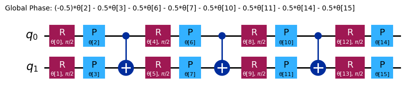
max_ansatz = QAOAAnsatz(max_hamiltonian, reps=2)
# Draw
max_ansatz.decompose(reps=3).draw("mpl")

# Sum the weights, and divide by 2

offset = -sum(edge[2] for edge in edges) / 2
print(f"""Offset: {offset}""")

Offset: -2.5

def cost_func(params, ansatz, hamiltonian, estimator):
    """Return estimate of energy from estimator

    Parameters:
        params (ndarray): Array of ansatz parameters
        ansatz (QuantumCircuit): Parameterized ansatz circuit
        hamiltonian (SparsePauliOp): Operator representation of Hamiltonian
        estimator (Estimator): Estimator primitive instance

    Returns:
        float: Energy estimate
    """
    pub = (ansatz, hamiltonian, params)
    cost = estimator.run([pub]).result()[0].data.evs
    #    cost = estimator.run(ansatz, hamiltonian, parameter_values=params).result().values[0]
    return cost

from qiskit.primitives import StatevectorEstimator as Estimator
from qiskit.primitives import StatevectorSampler as Sampler

estimator = Estimator()
sampler = Sampler()

초기 매개변수 집합을 무작위로 설정합니다.

import numpy as np

x0 = 2 * np.pi * np.random.rand(max_ansatz.num_parameters)
print(x0)

[6.0252949  0.58448176 2.15785731 1.13646074]

비용 함수를 최소화하기 위해 임의의 고전 최적화기를 사용할 수 있습니다. 실제 양자 시스템에서는 비평탄한 비용 함수 지형에 맞게 설계된 최적화기가 더 좋은 성능을 보이는 경우가 많습니다. 여기서는 SciPy의 minimize 함수를 통해 COBYLA 루틴을 사용합니다.

Runtime에 대한 반복적인 호출을 효율적으로 실행하기 위해 Session을 사용하여 모든 호출을 단일 블록 내에서 처리합니다. 또한 QAOA의 경우 해는 최소화를 통해 얻은 최적 매개변수로 바인딩된 ansatz Circuit의 출력 분포에 인코딩됩니다. 따라서 Sampler primitive가 필요하며, 동일한 Session으로 인스턴스화합니다. 최소화 루틴을 실행합니다.

result = minimize(
    cost_func, x0, args=(max_ansatz, max_hamiltonian, estimator), method="COBYLA"
)

print(result)

message: Optimization terminated successfully.
 success: True
  status: 1
     fun: -2.585287311689236
       x: [ 7.332e+00  3.904e-01  2.045e+00  1.028e+00]
    nfev: 80
   maxcv: 0.0

최적 매개변수 각도 벡터(x)를 ansatz Circuit에 대입하면 우리가 찾던 그래프 분할 결과를 얻을 수 있습니다.

eigenvalue = cost_func(result.x, max_ansatz, max_hamiltonian, estimator)
print(f"""Eigenvalue: {eigenvalue}""")
print(f"""Max-Cut Objective: {eigenvalue + offset}""")

Eigenvalue: -2.585287311689236
Max-Cut Objective: -5.085287311689235

from qiskit.result import QuasiDistribution
from qiskit.primitives import StatevectorSampler

sampler = StatevectorSampler()

# Assign solution parameters to ansatz
qc = max_ansatz.assign_parameters(result.x)

# Add measurements to our circuit
qc.measure_all()

# Sample ansatz at optimal parameters
# samp_dist = sampler.run(qc).result().quasi_dists[0]

shots = 1024
job = sampler.run([qc], shots=shots)

qc.decompose().draw("mpl")

data_pub = job.result()[0].data
bitstrings = data_pub.meas.get_bitstrings()
counts = data_pub.meas.get_counts()
quasi_dist = QuasiDistribution(
    {outcome: freq / shots for outcome, freq in counts.items()}
)
probabilities = quasi_dist

# Close the session since we are now done with it
# session.close()

from qiskit.visualization import plot_distribution

plot_distribution(counts)

binary_string = max(counts.items(), key=lambda kv: kv[1])[0]
x = np.asarray([int(y) for y in reversed(list(binary_string))])

colors = ["r" if x[i] == 0 else "c" for i in range(n)]
mpl_draw(
    G, pos=rx.shell_layout(G), with_labels=True, edge_labels=str, node_color=colors
)

요약

이번 강의에서 다음 내용을 학습했습니다.

• 사용자 정의 변분 알고리즘을 작성하는 방법
• 변분 알고리즘을 적용하여 최솟값 고유값을 구하는 방법
• 변분 알고리즘을 활용하여 응용 사례를 해결하는 방법

마지막 강의로 넘어가 평가를 완료하고 배지를 획득하세요!