핵 해밀토니안의 풀링된 샘플 기반 양자 대각화
사용량 추정: Nighthawk r2 프로세서에서 32초 (참고: 어디까지나 추정치이며 실제 실행 시간은 다를 수 있습니다.)
학습 목표
-
궤도의 -결합 기저로 표로 정리된 핵 껍질 모형 해밀토니안이, 하나의 큐비트가 하나의 단일 입자 상태에 해당하는 -스킴의 큐비트 해밀토니안으로 바뀌는 과정을 배웁니다.
-
각도가 2차 섭동 이론에서 나오는 고정된 비변분 들뜸 앤사츠를 구성하므로, 고전적 최적화 루프가 필요 없습니다.
-
큐비트 들뜸과 페르미온 들뜸을 비교하고, 이 선택이 앙상블의 2큐비트 깊이에 어떤 영향을 주는지 측정합니다.
-
보존량이 전자 수와 스핀이 아니라 핵자 수, , 그리고 패리티일 때
qiskit-addon-sqd로 자기 일관적 구성 복구를 실행합니다. -
정확하게 검증할 수 있는 24큐비트 문제에서 사용한 워크플로를, 이 튜토리얼의 정확 대각화 용량을 넘어서는 약 200만 개의 기저 상태를 가진 40큐비트 문제에 그대로 적용합니다.
사전 지식
시작하기 전에 다음 주제를 복습하세요.
-
화학 해밀토니안의 샘플 기반 양자 대각화: 이 튜토리얼의 전자 구조 대응편입니다.
-
2차 양자화와 조던-위그너 매핑.
배경
핵 껍질 모형은 원자핵을 비활성 코어 위의 작은 단일 입자 궤도 집합에서 움직이는 몇 개의 원자가 핵자로 취급하며, 측정된 스펙트럼에 맞춰 조정한 경험적 2체 힘을 통해 상호작용한다고 봅니다. 저에너지 핵 구조 연구에서 널리 쓰입니다. 계산 비용은 조합적으로 증가합니다. 기저는 원자가 양성자와 중성자를 사용 가능한 상태에 분배하는 모든 방법이고, 이 증가가 정확 대각화로 다룰 수 있는 모형 공간을 제한합니다.
풀링된 샘플 기반 양자 대각화(pooled SQD) [1]는 이 문제를 둘로 나눕니다. 양자 회로는 어떤 기저 상태가 중요한지 제안하는 데만 사용됩니다. 회로를 계산 기저에서 측정하면 측정된 각 비트열이 하나의 슬레이터 행렬식을 가리킵니다. 그런 다음 해밀토니안을 이 행렬식들이 생성하는 공간에서 고전적으로 구성하고 대각화합니다. 고전 단계는 부분 공간 안에서의 정확 대각화이므로 실제 바닥 상태 에너지에 대한 변분 상한을 돌려주며, 이 상한은 행렬식이 추가될수록 내려가기만 합니다.
이러한 역할 분담 덕분에 이 방법은 잡음에 강하지만, 중요한 한계가 있습니다. 잡음은 회로가 제안하는 행렬식이 어떤 것인지를 바꿉니다. 하지만 고전 해밀토니안에는 들어가지 않으므로 주어진 부분 공간의 고유값을 움직일 수는 없습니다. 보존량을 위반하는 샷은 버리거나 보정하고, 살아남은 샷은 어떻게 만들어졌든 유효한 기저 벡터입니다. 따라서 잡음은 정확성이 아니라 부분 공간의 품질을 떨어뜨리며, 어느 쪽이든 보고하는 값은 상한입니다.
핵 구조에는 샘플을 거를 수 있는 정확한 양자수가 여러 개 있습니다. 물리적인 행렬식은 올바른 수의 원자가 양성자 그리고 올바른 수의 원자가 중성자, 올바른 전체 각운동량 사영 , 올바른 패리티를 가져야 합니다. 각각은 비트열에 대한 정수 검사로 확인할 수 있습니다. 거부되는 샘플의 비율은 제약 조건과 모형 공간에 따라 달라집니다.
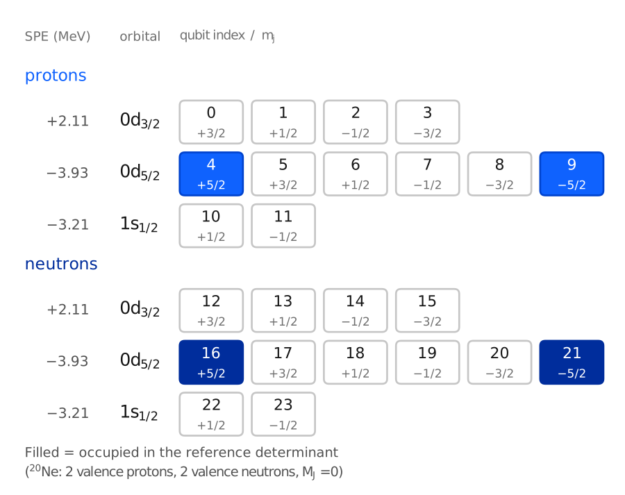
모든 큐비트는 하나의 -스킴 단일 입자 상태 이며, 은 점유됨을 뜻합니다. 레지스터는 고정된 순서를 사용합니다. 양성자가 먼저, 그다음 중성자 순이며, 같은 종류 안에서는 파일 순서대로 궤도를, 한 궤도 안에서는 내림차순으로 배치합니다. 따라서 비트열의 두 절반은 각각 양성자 구성과 중성자 구성입니다. 이는 풀링된 SQD 후처리 도구가 기대하는 이분할입니다.
워크플로
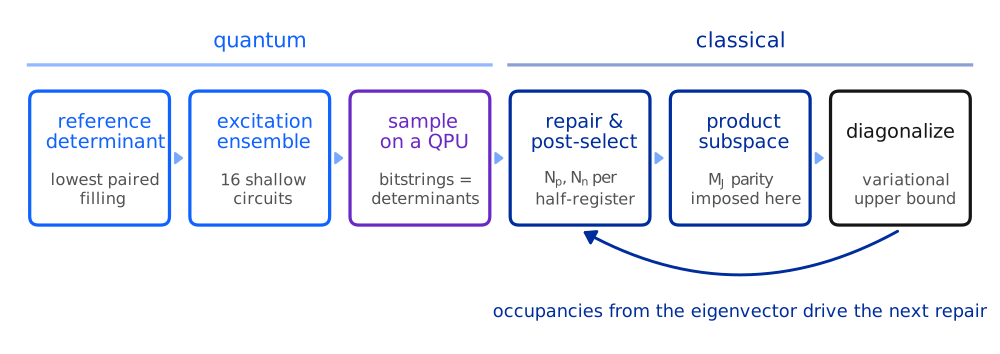
다이어그램의 두 단계가 핵 대칭성을 처리합니다.
보정과 사후 선택은 하드웨어 잡음의 영향을 받은 샘플을 처리합니다. 두 절반 레지스터의 핵자 수는 해밍 가중치이므로 qiskit-addon-sqd가 직접 처리합니다. recover_configurations는 샷을 버리는 대신, 평균 궤도 점유율의 현재 추정치와 가장 일치하지 않는 비트를 뒤집어 깨진 비트열을 보정합니다.
곱 부분 공간은 를 도입합니다. 은 두 절반을 결합하므로 어느 한쪽의 속성이 아니며, 따라서 전체 샷을 거르는 데 사용해서는 안 됩니다. 양성자 절반과 중성자 절반이 각각 유효한 비트열은 전체 가 틀렸더라도 두 개의 좋은 절반 구성을 제공합니다. 그러므로 부분 공간은 샘플링된 양성자 구성과 샘플링된 중성자 구성의 모든 곱으로 생성되며, 목표 와 패리티 섹터에 속하는 곱만 남깁니다. 이것이 풀링된 SQD의 부분 공간 구성이며, 수천 개의 비트열로 샘플 수보다 훨씬 큰 부분 공간을 생성할 수 있음을 뜻합니다.
두 가지 지배 방정식
껍질 모형 해밀토니안은 1체 항과 2체 상호작용의 합입니다.
여기서 는 -스킴 상태를 나타내며 은 양성자, 은 중성자입니다. USDA [2]와 GXPF1 [3] 같은 경험적 상호작용은 -스킴이 아니라 -결합 기저에서, 궤도 의 정규화된 반대칭 2체 상태 사이의 행렬 원소 로 표로 정리되어 있습니다. -스킴 원소를 복원하는 것은 클렙슈-고르단 재결합입니다.
인자는 표로 정리된 상태의 정규화 규약을 되돌립니다. 이 튜토리얼의 나머지는 모두 이 두 방정식을 바탕으로 합니다.
세 가지 실행
| 핵 | 껍질 | 큐비트 | 대칭성 허용 기저 | 정확히 검증 가능? | |
|---|---|---|---|---|---|
| 소규모 | (2p + 2n) | 24 | 640 | 예 | |
| 대규모 | (2p + 2n) | 40 | 4,000 | 예 | |
| 대규모 | (4p + 4n) | 40 | 1,963,461 | 아니요 |
소규모 실행은 따라 하기용 예제입니다. 두 대규모 실행은 모두 40큐비트 레지스터를 사용합니다. 첫 번째는 노트북에서도 정확하게 대각화할 수 있을 만큼 작아서 하드웨어 결과를 정확한 기준값과 비교할 수 있습니다. 두 번째는 이 튜토리얼의 정확 대각화 용량을 넘어섭니다.
여기의 모든 실행은 QPU에서 수행됩니다. 이는 방법의 요구 사항이 아니라 이 튜토리얼을 위한 선택입니다. 세 실행이 같은 백엔드와 게이트 예산을 공유하므로 문제 크기별 성능을 비교할 수 있습니다.
요구 사항
시작하기 전에 다음 패키지를 설치하세요.
-
Qiskit SDK v2.0 이상 (
pip install qiskit) -
qiskit-ibm-runtimev0.40 or later (pip install qiskit-ibm-runtime) -
SQD 애드온 v0.12 이상 (
pip install qiskit-addon-sqd) -
NumPy, SciPy, Matplotlib (
pip install numpy scipy matplotlib)
또한 로컬에 자격 증명이 저장된 IBM Quantum® 계정과, 40큐비트 이상의 QPU에 대한 접근 권한이 필요합니다.
시뮬레이터 패키지는 필요 없고, 내려받아야 할 데이터 파일도 없습니다. 이 튜토리얼에서 사용하는 두 상호작용 파일은 다음 설정 셀에 포함되어 있으며, 셀을 실행하면 임시 디렉터리에 기록됩니다.
설정
이 섹션에서는 도구를 가져오고, 워크플로가 사용하는 순서대로 워크플로에 필요한 껍질 모형 헬퍼를 정의합니다. 각 헬퍼의 배경이 되는 물리는 부록에서 유도하며, 주석에서는 각 함수가 워크플로에서 맡는 역할을 설명합니다.
먼저 두 상호작용 파일의 압축을 풉니다. 둘 다 공개된 매개변수 집합이며, 노트북이 독립적으로 동작하도록 여기에 포함했습니다. usda.snt는 USDA -껍질 해밀토니안 [2]이고 gxpf1.snt는 GXPF1 -껍질 해밀토니안 [3]입니다.
# Added by doQumentation — installs the packages this notebook needs if they are missing
import importlib.util

_needed = {"matplotlib": "matplotlib", "numpy": "numpy", "qiskit": "qiskit", "qiskit_addon_sqd": "qiskit-addon-sqd", "qiskit_ibm_runtime": "qiskit-ibm-runtime", "scipy": "scipy"}
_missing = [pip for module, pip in _needed.items()
            if importlib.util.find_spec(module) is None]
# One at a time, so a package that fails to install does not block the others
for _pip in _missing:
    %pip install -q {_pip}
if not _missing:
    print("\u2713 All required packages are installed")
from __future__ import annotations

import base64
import gzip
import itertools
import tempfile
from dataclasses import dataclass
from functools import lru_cache
from math import factorial, sqrt
from pathlib import Path

import matplotlib.pyplot as plt
import numpy as np

from qiskit import QuantumCircuit
from qiskit.circuit.library import PauliEvolutionGate
from qiskit.quantum_info import Operator, SparsePauliOp
from qiskit.transpiler.preset_passmanagers import generate_preset_pass_manager
from qiskit_addon_sqd.configuration_recovery import recover_configurations
from qiskit_addon_sqd.counts import bit_array_to_arrays
from qiskit_addon_sqd.subsampling import postselect_by_hamming_right_and_left
from qiskit_ibm_runtime import QiskitRuntimeService, SamplerV2

from scipy.linalg import eigh

_USDA_SNT_GZ = (
    "H4sIAI5wqWoC/4WY224bRwyG7/UU9F0CONsZco5AUyBuC/QmQNG06KWhWGql1LYMy+kJefiOTrucGXJrQAgsf5nl8ecOr+CX"
    "D9+9g/0K9pv1/T389rx7gPLrsH+Cz/vVctg+vgAsrgB+HeDdAD9t7zYv6+dr+DDA+z8223/X17B8XMFN+ev9+m+4ed799XjA"
    "f9z8sy/4+s8BvoWYrsEERwbhFRqTXi+uCvOwW63vYf+0vFvDAgDo/AFIh8/hK7DH30354Omvb8o3V8c/vIUnMKtboK/wiGKF"
    "+gnFEfVn9PQUe8bthNIRtftbsGfUtQbAGXUFfawM8K0BF9SP6MWA0BpwQcMRvRhwBSX86+fl3ct2d4jq4+eHa3hYv2x2q7fX"
    "AJuPy+fb3cP69+Uh4luAT8djv95++eGV/fj6y6dvFudnmcX4lGOoBmttNOVncTL2FLs3NGT0l++ndJTv0cR8/t6NUanP8WMI"
    "6nPC6C8/5wp+vnn//QLOP9ank3k2wRszkDn/Zwv15xiv41l2SDmjhuEFM4PJ0QkYcgzM4A1Jp1GDkcvtaWMAR9tosAa9huHk"
    "AtoUBYwaF8hGarAxOywgxnoeN+Se2smF4H3QMPZQ653XMJpOi6GyrcLcZJtzLgoYcdsOyXKibV1Aom0fikJO0VLUMDeW3kAl"
    "qQLWpd66qGE02eZ9lXqSPD3UWyl5DeOeGnINJnmaUggCVrtgh2DJNm3fVy8WF3LSMFa9hYga5iYX0IQsYK2nmTpJkoq81Acy"
    "jLTTnPEaxqo3JGcbvZMeGnJVbw6mf2cUqcIsO80nFdOFq8JoSlY+Zb7FfNNZlnw2PqOE8SL3PtlSJhJGXGqsDRjbh4bmocWy"
    "oiIxSxjv09JYgaxlGLZxA9EFFOImuIBt3EB04TK3Z5S8wizrrFCJQ4Xpgl9hzDYbu0LCNm6HzkJHweUkYazITalyF7NjGAnh"
    "FZJFQniFZFHnqWgbdZ6qtoX50VZhvEJ81TJe7AUcQozH8yQMJ8ymUS07jLin6LXT3FRIhmwSTmtbJpEjr2AsvM7E1ra+ZaiM"
    "NoxewZinBlPQTmPJyikn7TQ2630SbWuz4CLlwzuGhCHPqbUmRZQwpkiBDn1vsoQ55oKjbEvNNVgbXls0WvA0NKnPpku91Fkx"
    "pahhXPDJtxVCQkBcMtJD27I8VJGAhWYYlVuZzc5e+jSIZWnLa57nOQ1iWZY+jSE3GP5/QIKi5E1Agqi9BbMZiUjEWNwChqKq"
    "KTZY11ku5ca2Pqc4YKk1o2DstBjJC1htW2nAgEZ4aDdPvQmmmLeY4tWFt9Y3VAdlpW+oDcpa3zpM1jdUB2XV9agOyqrrcWZQ"
    "sq7vMMffBseux5l5yjoLZ+Yp6yzU5mmt5DgzT5mSozZPoVIknJmnTJFQHZRV12OrlvpFQFbycoGKOWiYfl9QlXySGtSUvL9W"
    "VJi/YG4grC4CmuCX6CZrKUsY64UyJolCQoZJqWeKhDOCzxQJNcGXbZMEX7EtzF+gvCI1npxjmKaW5Q06ewVjOY0u2+Y0kt5D"
    "JhlETS2P+5CqyIMYkCI1NK50SO3TarSR2qfVaKOZPmXjg2beVJmS01zqp/CSmvoqvNSOD/kaS+qUoSGaTM2yz83fdjtMvsZy"
    "xOv7N44Fff/GT5q5tXWYfB3jWND3b9yumUvK5SQnvK6w/VuHyfu3DpP3bx0m7984FvT9W4fJ+zceWq/v3zpM3r9xLOj7tw6T"
    "928X053QgGz/1mHy/u3yZ8lTtn/jWND3b74NiDx2vRbeep56Lbz1oPRaeOv9G0dmxofXPK33bx0m798C1B9RuP4DPJ0WcLAa"
    "AAA="
)

_GXPF1_SNT_GZ = (
    "H4sIAI5wqWoC/4WcQY8dtw3H7/kU41sCeF8lUqKkQw9NgbaXoEHQQ26BkdiIEWdt2E6L9tNXb9+ORIn8PwdZILB/S3I4IsW/"
    "ZiYvjr//+P3f4nG8ef/x+PDm4dOvr9+9++rF8d3l+Mf7x99fvTz+dTn++fnTH7/1//z28pfL8e3H9/95fHm8evzl+lffvf3f"
    "H59e/fb26L9zHN//+t9Pl+OH1/++HH89JL88gkQO8esfvjm+phDomyvW//39/S+v3x2fPrz6+fVX/dfS889B4fpz/aN43P7p"
    "f3Bw/ynH8fD0Zy+uf/fn48MR3vxU/kRXlp7Z+PzDiqUnNn74iW8sb3azYvm0m29s2uxGxabTbryx2cZ7nGzu7KOKV2y8g5Un"
    "dsZbbLyDLafd53irjXew9bR7jffF8fbx8+uPr37+/Pb941dPv3P93ZH4W/If6kUohXCm+Jbmh3yR0jicybwl9CFeuFILy908"
    "HtIlcrlZyCNJ2q6MdGi7ZVy4tlvHJS52Y71FnHp8D+HCIYTlQuYFhdsv0yVxzZB6vsxwaZwJUumkIjWB1POdDhcqlR2KVo85"
    "SoDU8NgdNodiZevqMUqB1LCVWsO2ZMQlyYs+bXEFk4m5bMJJlVgSpGjaouhQvFKxUIbUjIvI85hWW4FNvubyDnMxMkFKRc8V"
    "Uml65OhQW1x9fe3XOAtsZPXJ36TIX18SaoQUnysnZsHUXPfcKqTyaSu36FHbWg0tN0jxWIXEAVLzbqcqkMpj3T8lwlBp9RhD"
    "qpAaHpnzni9nRXPh6lDbysmJBVLzDtU71KztnDxqW1+JhDaKnTtUa4DUzH00Hp0VXQMHSM3c16irlpf7GEcN1dogpfpEDpAa"
    "WRUOBKl0UqkIQ2qs+5IYU6OvthbFodIaF6/9i51VeF0TLZSN2lfh9T729utQOqtXKi/dl/21mihhW+M+BpIKqblypDWHSntc"
    "mSA1O3nMe+6dHp0DEaRmXCU0h9p7dOYCqVm1MehOnvy7nWphSKnuu+Q++X2Ca4uQGrYkxp3yMkFLL0ygavPovmR64dhFY5QM"
    "KVK1XRxqX4UydlHCXU44hY1ydndKuUBK11BzqH1NNOKNMvt27PMXVUWBemSqCVIjrr4nYFtzTSQJkJp3O7se09p9YygCKVL7"
    "UN4opx5DNnE5q5AlerZ2jyExpEYmggTtMYFrzC1Bak58jetGeSvHenSip9ROik0m5lqdsxzjrCYhTM1uImOHYZzVPvnWjXIm"
    "0RoaKyqhjjlqiEE3uWoYHqopbT/KY0pDD+Xtx9d8lvI0n6U8zWcpT/NpQqDms5Sn+TRVoOazlKf5LOVpPk1VqPl05AI1n6U8"
    "zaepAjWfpTzNp6kKNZ/OQoGaz1Ke5rOUp/k0VaHm03mvUPOd1+esL6X5LOVpPkt5ms9SnubTVIGaz1Ke5rOUp/ks5Wk+TVWo"
    "+SzlaT69mgVqPk0VqPks5Wk+S3maT1MVaj5dPwVqPkt5mk9TFWo+S3ma77x/8z56ms9SnuazlKf5LOVpPkt5ms9SnubTVIWa"
    "z1Ke5jupfRWumk9TBWo+S3maz1Ke5rOUp/k0VaHms5Sn+XTnLVDzWcrTfJqqUPNZytN85/1z7rbSfJbyNN/5t06fUJrPUp7m"
    "OykvE7T0wgqqdmo+Mb3Q03yCO6bSfII7ptJ8gruc0nxi+pen+eROL5yaT3CXU5pPx1Sh5hNcj0rzCajHVfMJqMdV88mdesyu"
    "xwo1n+B6VJpPcD0qzSe4HpXmE1yPSvMJrkelwERVR4Waz1Ke5hNTQ3THoxO90nzFZMLTfAVnVWm+grOqNF/BWVWaTxMVar6C"
    "r1FpvgK6yar56vbja76onormu8/5ViqOrNblZH6l0NPAlRq9sKaIbaFnhis15tUuH/E1oieLK1XOTIgsz3ROap9XpQ/SJWqK"
    "bCYcKm6K4tp9iUqqzbd1j4qO+g2tpTV6sll1qLipk6fnw32/isDWPSruPborwz7x9eakKbbry6Gi7RN9nrhuHr4tPXXsVLT9"
    "vvTdKlUQ18i9Q0Wn+2ZOlYpva0yiDhXthNz69p4S+7ZG7h0q2jma+/BIIfm2RnU4VLQ9R6hG4iWryVurhorOlNbzEJr4tubk"
    "bim6e25iqbFbJY4MKfREfaXGNXKK2aF2BSapD6Oy5162yd1S5Og0iq3k5tua1WEpsus+ZO4ZS76tqU4sRc7+mAtJyL6teR8t"
    "RVbDUO9yXM2a2O6jQ5GjdCi3HKpva04dluK7J1uWGtFLjhFS6J2HlZpKhzOm0JsRK5XnmjD7Izv5av0eBd7zVb5IsVU6ffTN"
    "oQXf1peoeveNjZWaNURFZ0L8fTsX1s9hwO4eeHkOA3Z3Zct6ZOccgPAM0O91hR4ZPEcWMAPkdBWQvsdZj72xZuTRs2U95qFY"
    "a8FZHVQpy/Mhd55YbGmPew2VGB2PRvOVsNlib0orYbO1U8fi0cbF6uQhw7jUycMybYs/dSiKwGxyLB5tXEmdM5WM4lKnGLFm"
    "FFeaPTruK8ehlEcbV55n2yIwrnlOXorAuPKsxyIwrjz7l3greptzSgve+tqo2lLbcu9MQ4oiPDMpjzaueR8rUUZxqaql/T46"
    "k5WiCM9fyuNpy5uZpM9WkvfaxpS1Ndd96JKV2LflUdrW1idaKOT0HNMnTCdnT/OZvcOZv5RHG5fqAJFhXLO2WykwrtlzJkV4"
    "llMebVxp7kOUMopr7h1dSmcUl9LuxesT2z6kPOq4ttkkk7sj1/1JWWWnHvfdfVKE50LlUV+jObPqs2hO+zViytpSJ+CFSyu+"
    "LY+yttRM3gf3HH1bHmVtzR5NXZQXcI0epW1tdyh2d86a2O52F9vR6V8FUgTm1dWjjWuepZUgMK45k2cKMC6PIjD7rh6j+gpi"
    "0Y904b675/n2h3u6QteTedkoc7qy2LIeaUxpkXNAHgeV53khozOYxZb1qDpTrvAa+TxBClECvEbPlvWY5o4cA7zGNDSfFIbX"
    "6NmyHmd1SEnwGgfVJ6YKr9GzZT3KebdDZIYe5bzGQLFAj54t7XHXfDkmJ6v789r17e7iTEMrxXhmUh5tXHNmainCuObMVBOO"
    "y6MYzEyrx9MW2VMf4cC9NWlbzpmVoqytucPkIO12SsZ4/lKUtTX7V6LGsfi2phadlLa1nX89naUHc437uYnQni/nlEzWN/S8"
    "s7TVo41LvUsW9+pwqFBl79HsPYkVr/sK9GjjYnVWSzBfqjoowXx5FN+ZC6dHG5d6WybjfM15ouYE8+VRDObC1aOOa3v+WEJq"
    "Tlzb2VCRELOtbYEU47NH5dHGpd5nagzj0s+HAozLoxjMq6tHnfutHmNjblz23G/1qChra3rMOT6f3jGefRVlbamZKfR1COKa"
    "PWdS1tZcXy3mnMm3pd4IGpS1Nd9Uai0Wir6t+fxxUtrWPvu27M1MG8XJ1KMz+yqK8Vmt8mjjmn1CKmcUF88zhVIzimtOtZNi"
    "fO6rPGpbW9XGLrg50G5rfwNhUueu7swmEtI55yQ0m/RpqI3JPd15ujVtWY9TSbcxpSU8dSShAj16tk4b3r6dmUlI2/L27Ulp"
    "W7vKLFK3uByK4nI2VP19SFEJ7EOrRxvXyESr413YhPchLsssV/0dRlEJ70PKo7a1n/vWa1rLbsu8mTooa0up8tpyEd+Wep42"
    "KG1rf6su5ebkvpqztLzl3qltRSVc28ojmTM+9F2TwNm3Qgp9/eSeKnaNXFtwqH3nk1KaJE05M6ZDOdNjv9NJIvm2Zr+3lFeP"
    "EvqGnH1bM/eWMtNQvFCRHnzUlJlzXMqZYFKqHHLxbdFUFIbiu+8XWmo+50vL6R06l1u/PBO/asN8B5zAmdXTDtP7r8h+jeWL"
    "lFOPocYumti39SWq3v0iTvxdtDw9hhmUq9N6PbaqvzJyqyNeMi0nIm51LLbojgIrOUKP+l2yBj16tghrqxib1gqg0pLknfIq"
    "bdoirJqkMMNrnDNATPgaPVuE9VBv0J7HbU107V42W44eUhSjPrF4JKyHUokZxqXeTV+exAI9pCjGp/zKIwE9dO2+XSTX1vbc"
    "b6pJUYT1UOCWWw2+rdmZJkVYD1Ef0Uoi39acySdFWA9RztLVjm9LPQ0cFAENc3unJjrVsWuY0mK297EYxbrbcs7vlUfCGib3"
    "bQ/GNWffMijCGkZRDHr0w+KRsIbpnem6dnZbe9VOitTsW7e3I+e7Pgnv7tfHQxvl7O7KlvU4zu95fouUUNV21RSGFk2oHhdb"
    "ZGbf+b4cXf8nRlnb8maASVlbc+UkSnSb0hKox4eFIjNHz7c/aHydkvC6T9Lydo3Je+u8ZSdf+xsu06O2ta2vPr70W1l2W9v6"
    "UhSbPoG+kwYnSDVnTKGvqYvfv3JuDVLom2vvpOZpvh9fizHuX71jVp79vqDcG8rrJolLnecTxe8TgMLfBTDoJteOGUVntYJr"
    "5PHOVsKnUaEuJw8oE9MWA5V5e2tA9wmQrw5xQB6RrernS33VkEB1PCmKW5f7P6zudeW7TwAA"
)

DATA = Path(tempfile.mkdtemp(prefix="nuclear_sqd_"))
for name, blob in (("usda.snt", _USDA_SNT_GZ), ("gxpf1.snt", _GXPF1_SNT_GZ)):
    (DATA / name).write_bytes(gzip.decompress(base64.b64decode(blob)))

    if not (DATA / name).is_file():
        raise RuntimeError(f"{name} did not unpack to {DATA}")
모형 공간과 큐비트 레지스터
.snt 파일에는 모형 공간, 단일 입자 에너지, -결합 2체 행렬 원소가 들어 있습니다. 여기서 사용하는 질량 의존 상호작용의 경우, 2체 헤더의 세 번째와 네 번째 필드가 상호작용을 맞춘 기준 질량 와 질량 의존성의 지수를 지정합니다. 두 파일 모두 지수 을 가지며 는 USDA에서 , GXPF1에서 이므로, 표로 정리된 행렬 원소는 계산 대상 핵에 맞게 으로 재조정해야 합니다 [2], [3]. 단일 입자 에너지는 재조정하지 않습니다. 이 단계를 건너뛰면 상관 에너지가 몇 퍼센트 달라집니다.
이어서 나오는 에너지는 비활성 코어를 기준으로 측정한 원자가 에너지이며, 실험적인 분리 에너지가 아닙니다.
@dataclass(frozen=True)
class Orbital:
    idx: int
    n: int
    ell: int
    j2: int
    tz: int  # j2 = 2j; tz = -1 proton, +1 neutron

@dataclass(frozen=True)
class SPState:
    """One m-scheme single-particle state, i.e. one qubit."""

    orb: int
    j2: int
    mj2: int
    tz: int
    ell: int
    spe: float  # mj2 = 2 * m_j

@dataclass
class ModelSpace:
    orbitals: list
    spes: dict
    tbmes: dict
    core_z: int
    core_n: int
    mass_number: int
    a_ref: int
    mass_exponent: float
    mass_factor: float

def read_snt(path, n_protons, n_neutrons):
    """Parse a .snt interaction file, applying its mass dependence for this nucleus.

    The two-body header line is ``n_tbme  method  A_ref  exponent``.  When ``method`` is 1 the
    tabulated matrix elements are rescaled by ``(A / A_ref) ** exponent``, where A is the mass
    number of the whole nucleus -- the core plus the valence nucleons.  A is derived from the
    file's own core numbers rather than passed in, so it cannot silently disagree with the
    valence counts the rest of the workflow uses.  Single-particle energies are not rescaled.
    """
    rows = [
        ln.split("!")[0].split() for ln in Path(path).read_text().splitlines()
    ]
    rows = iter([r for r in rows if r])

    n_p_orb, n_n_orb, core_z, core_n = (int(x) for x in next(rows)[:4])
    orbitals = [
        Orbital(*(int(x) for x in next(rows)[:5]))
        for _ in range(n_p_orb + n_n_orb)
    ]

    spes = {}
    for _ in range(int(next(rows)[0])):  # "i  i  <i|H(1b)|i>"
        field = next(rows)
        spes[int(field[0])] = float(field[2])

    n_tbme, method, a_ref, exponent = next(rows)[:4]
    n_tbme, method, a_ref, exponent = (
        int(n_tbme),
        int(method),
        int(a_ref),
        float(exponent),
    )
    mass_number = core_z + core_n + n_protons + n_neutrons
    factor = (mass_number / a_ref) ** exponent if method == 1 else 1.0

    tbmes = {}
    for _ in range(n_tbme):  # "a  b  c  d  J  value"
        field = next(rows)
        tbmes[tuple(int(x) for x in field[:5])] = float(field[5]) * factor

    return ModelSpace(
        orbitals,
        spes,
        tbmes,
        core_z,
        core_n,
        mass_number,
        a_ref,
        exponent,
        factor,
    )

def m_scheme_states(ms):
    """The qubit register: protons then neutrons, orbitals in file order, m_j descending."""
    return [
        SPState(o.idx, o.j2, m2, o.tz, o.ell, ms.spes[o.idx])
        for tz in (-1, +1)
        for o in ms.orbitals
        if o.tz == tz
        for m2 in range(o.j2, -o.j2 - 1, -2)
    ]
클렙슈-고르단 재결합
식 (2)에는 반정수 각운동량에 대한 클렙슈-고르단 계수가 필요합니다. 모든 인자는 물리적 값의 두 배로 전달되므로, 는 5로 들어가며 산술이 정확하게 유지됩니다.
Interaction.v_ms는 상호작용 행렬 원소의 조회를 처리합니다. .snt 파일은 각 행렬 원소를 한 번만 저장하므로, 조회 시 어느 쪽에든 반대칭화된 쌍 교환 위상 가 필요할 수 있고, 브라와 켓이 어느 순서로 저장되어 있을 수도 있습니다.
@lru_cache(maxsize=None)
def clebsch_gordan(j1_2, j2_2, J_2, m1_2, m2_2, M_2):
    """<j1 m1 j2 m2 | J M>.  Every argument is twice its physical value."""
    if m1_2 + m2_2 != M_2 or not abs(j1_2 - j2_2) <= J_2 <= j1_2 + j2_2:
        return 0.0
    if abs(m1_2) > j1_2 or abs(m2_2) > j2_2 or abs(M_2) > J_2:
        return 0.0
    if (j1_2 + j2_2 - J_2) % 2 or (j1_2 - m1_2) % 2 or (j2_2 - m2_2) % 2:
        return 0.0

    f, half = factorial, lambda x: x // 2
    prefactor = sqrt(
        (J_2 + 1)
        * f(half(j1_2 + j2_2 - J_2))
        * f(half(j1_2 - j2_2 + J_2))
        * f(half(-j1_2 + j2_2 + J_2))
        / f(half(j1_2 + j2_2 + J_2) + 1)
        * f(half(J_2 + M_2))
        * f(half(J_2 - M_2))
        * f(half(j1_2 - m1_2))
        * f(half(j1_2 + m1_2))
        * f(half(j2_2 - m2_2))
        * f(half(j2_2 + m2_2))
    )
    total = 0.0
    for k in range(half(j1_2 + j2_2 - J_2) + 1):
        d = [
            half(j1_2 + j2_2 - J_2) - k,
            half(j1_2 - m1_2) - k,
            half(j2_2 + m2_2) - k,
            half(J_2 - j2_2 + m1_2) + k,
            half(J_2 - j1_2 - m2_2) + k,
        ]
        if all(x >= 0 for x in d):
            total += (-1) ** k / (
                f(k) * f(d[0]) * f(d[1]) * f(d[2]) * f(d[3]) * f(d[4])
            )
    return prefactor * total

class Interaction:
    """Antisymmetrized m-scheme two-body matrix elements <pq||rs>, per Eq. (2)."""

    def __init__(self, model_space, sp):
        self.ms, self.sp, self._cache = model_space, sp, {}

    def _tbme(self, oa, ob, oc, od, J, j_ab_2, j_cd_2):
        """<oa ob; J|V|oc od; J>, allowing for how the file happens to order each pair."""
        table = self.ms.tbmes
        # |ba; J> = -(-1)^(j_a + j_b - J) |ab; J> for a normalized antisymmetrized pair;
        # dropping the leading minus makes v_ms symmetric instead of antisymmetric, and
        # the Hamiltonian then fails the rotational-invariance check in Step 1.
        phase_ab = -1.0 if (j_ab_2 // 2 - J) % 2 == 0 else 1.0
        phase_cd = -1.0 if (j_cd_2 // 2 - J) % 2 == 0 else 1.0
        for keys, phase in (
            (((oa, ob, oc, od), (oc, od, oa, ob)), 1.0),
            (((ob, oa, oc, od), (oc, od, ob, oa)), phase_ab),
            (((oa, ob, od, oc), (od, oc, oa, ob)), phase_cd),
            (((ob, oa, od, oc), (od, oc, ob, oa)), phase_ab * phase_cd),
        ):
            for key in keys:
                value = table.get(key + (J,))
                if value is not None:
                    return value * phase
        return 0.0

    def v_ms(self, p, q, r, s):
        """<pq||rs>, zero unless M_J and charge are conserved."""
        cached = self._cache.get((p, q, r, s))
        if cached is not None:
            return cached

        P, Q, R, S = (self.sp[i] for i in (p, q, r, s))
        value = 0.0
        if P.mj2 + Q.mj2 == R.mj2 + S.mj2 and P.tz + Q.tz == R.tz + S.tz:
            M = P.mj2 + Q.mj2
            # sqrt(1 + delta): undo the normalization of the tabulated pair states
            c12 = sqrt(2.0) if (P.tz == Q.tz and P.orb == Q.orb) else 1.0
            c34 = sqrt(2.0) if (R.tz == S.tz and R.orb == S.orb) else 1.0
            for J2 in range(
                max(abs(P.j2 - Q.j2), abs(R.j2 - S.j2)),
                min(P.j2 + Q.j2, R.j2 + S.j2) + 1,
                2,
            ):
                cg_bra = clebsch_gordan(P.j2, Q.j2, J2, P.mj2, Q.mj2, M)
                cg_ket = clebsch_gordan(R.j2, S.j2, J2, R.mj2, S.mj2, M)
                if abs(cg_bra) < 1e-12 or abs(cg_ket) < 1e-12:
                    continue
                value += (
                    c12
                    * c34
                    * cg_bra
                    * cg_ket
                    * self._tbme(
                        P.orb,
                        Q.orb,
                        R.orb,
                        S.orb,
                        J2 // 2,
                        P.j2 + Q.j2,
                        R.j2 + S.j2,
                    )
                )

        self._cache[(p, q, r, s)] = value
        return value
행렬 원소와 대칭성 검사
행렬식은 점유된 큐비트 인덱스의 정렬된 튜플입니다. 점유된 상태가 두 개를 넘게 다른 두 행렬식은 행렬 원소가 0이 됩니다. 그렇지 않으면 슬레이터-콘돈 규칙에 따라 상호작용에 대한 짧은 합이 나오며, 여기에 고정된 레지스터 순서에서 연산자 사이에 점유된 상태가 몇 개 있는지를 세는 페르미온 부호가 곱해집니다.
symmetry_allowed는 네 가지 정확한 양자수가 모두 귀결되는 정수 검사입니다. 샘플을 거르는 데 쓰이고, 정확하게 검증할 수 있을 만큼 작은 실행에서 정확한 기저를 나열하는 데도 쓰입니다.
def matrix_element(inter, det_a, det_b):
    """<A|H|B> for two determinants, each a sorted tuple of occupied qubit indices."""
    set_a, set_b = set(det_a), set(det_b)
    out_a, out_b = sorted(set_a - set_b), sorted(set_b - set_a)
    if len(out_a) != len(out_b) or len(out_a) > 2:
        return 0.0

    if not out_a:  # diagonal: one-body plus two-body
        return sum(inter.sp[i].spe for i in det_a) + sum(
            inter.v_ms(i, j, i, j)
            for i, j in itertools.combinations(det_a, 2)
        )

    if len(out_a) == 1:  # one state moves, p -> q
        p, q = out_a[0], out_b[0]
        crossings = sum(1 for k in set_a if min(p, q) < k < max(p, q))
        return (-1.0) ** crossings * sum(
            inter.v_ms(p, j, q, j) for j in det_a if j not in (p, q)
        )

    (p, r), (q, s) = out_a, out_b  # two states move
    crossings = sum(1 for k in set_a if p < k < r) + sum(
        1 for k in set_b if q < k < s
    )
    return (-1.0) ** crossings * inter.v_ms(p, r, q, s)

def subspace_hamiltonian(inter, dets):
    """Dense real-symmetric H projected onto the span of `dets`."""
    H = np.zeros((len(dets), len(dets)))
    for a, det_a in enumerate(dets):
        H[a, a] = matrix_element(inter, det_a, det_a)
        for b in range(a + 1, len(dets)):
            H[a, b] = H[b, a] = matrix_element(inter, det_a, dets[b])
    return H

def ground_state(inter, dets):
    """Lowest eigenvalue and eigenvector of H over `dets`."""
    values, vectors = np.linalg.eigh(subspace_hamiltonian(inter, dets))
    return values[0], vectors[:, 0]

def symmetry_allowed(
    sp, det, n_protons, n_neutrons, mj2_target=0, parity_target=0
):
    """The four exact shell-model quantum numbers, as integer tests on one determinant."""
    n_p = sum(1 for i in det if sp[i].tz == -1)
    return (
        n_p == n_protons
        and len(det) - n_p == n_neutrons
        and sum(sp[i].mj2 for i in det) == mj2_target
        and sum(sp[i].ell for i in det) % 2 == parity_target
    )

def full_basis(sp, n_protons, n_neutrons, **targets):
    """Every symmetry-allowed determinant.  Only tractable for small model spaces."""
    protons = [i for i, s in enumerate(sp) if s.tz == -1]
    neutrons = [i for i, s in enumerate(sp) if s.tz == +1]
    return [
        p + n
        for p in itertools.combinations(protons, n_protons)
        for n in itertools.combinations(neutrons, n_neutrons)
        if symmetry_allowed(sp, p + n, n_protons, n_neutrons, **targets)
    ]

def count_basis(sp, n_protons, n_neutrons, mj2_target=0, parity_target=0):
    """How many determinants `full_basis` would return, without enumerating them.

    A dynamic program over (occupied count, sum of 2*m_j, parity) per species.  This stays
    cheap when the basis itself is far too large to build, which is how the largest run below
    can report the size of the space it is sampling from.
    """

    def species(states, k):
        table = {(0, 0, 0): 1}
        for s in states:
            for key, value in list(table.items()):
                count, m_sum, parity = key
                if count < k:
                    nxt = (count + 1, m_sum + s.mj2, (parity + s.ell) % 2)
                    table[nxt] = table.get(nxt, 0) + value
        totals = {}
        for (count, m_sum, parity), value in table.items():
            if count == k:
                totals[(m_sum, parity)] = (
                    totals.get((m_sum, parity), 0) + value
                )
        return totals

    left = species([s for s in sp if s.tz == -1], n_protons)
    right = species([s for s in sp if s.tz == +1], n_neutrons)
    return sum(
        a * b
        for (mp, pp), a in left.items()
        for (mn, pn), b in right.items()
        if mp + mn == mj2_target and (pp + pn) % 2 == parity_target
    )
기준 행렬식
앤사츠는 하나의 행렬식 위에 구성되므로, 그 행렬식은 사용 가능한 것 중 최선이어야 합니다. 가장 낮은 단일 입자 에너지를 채우는 방식은 2체 상호작용을 무시합니다. 이런 모형 공간에서는 그 선택이 최저 에너지 행렬식보다 1–2 MeV 높은 에너지를 줍니다.
시간 반전된 쌍으로 이루어진 채움으로 제한하면 이 정확히 강제되고 종류당 후보가 개(많아야 수천 개)만 남으므로, 전체 대각 성분 로 모두 탐색하여 최선의 것을 찾을 수 있습니다. 동점이면 쌍 형성력이 가장 강한, 가장 강하게 정렬된 쌍을 택합니다. 이 튜토리얼에서 전체 열거와 대조해 확인할 수 있는 모든 경우에, 탐색은 전역 최저 대각 성분 행렬식을 반환하며, 이는 정확한 바닥 상태의 가장 큰 단일 성분이기도 합니다.
def reference_determinant(sp, inter, n_protons, n_neutrons):
    """Lowest-diagonal determinant built from time-reversed (+m_j, -m_j) orbital pairs."""
    if n_protons % 2 or n_neutrons % 2:
        raise ValueError(
            "an odd valence count has no time-reversed paired reference at M_J = 0"
        )

    def species_pairs(tz):
        return [
            (
                q,
                next(
                    p
                    for p, t in enumerate(sp)
                    if t.tz == tz and t.orb == s.orb and t.mj2 == -s.mj2
                ),
            )
            for q, s in enumerate(sp)
            if s.tz == tz and s.mj2 > 0
        ]

    best = None
    for chosen_p in itertools.combinations(species_pairs(-1), n_protons // 2):
        protons = tuple(q for pair in chosen_p for q in pair)
        for chosen_n in itertools.combinations(
            species_pairs(+1), n_neutrons // 2
        ):
            det = tuple(
                sorted(protons + tuple(q for pair in chosen_n for q in pair))
            )
            # break ties toward the most aligned pairs, where J = 0 pairing is strongest
            score = (
                matrix_element(inter, det, det),
                -sum(abs(sp[q].mj2) for q in det),
            )
            if best is None or score < best[0]:
                best = (score, det)
    return best[1]
들뜸 풀과 섭동적 순위 매기기
상관은 기준 상태로부터의 2입자–2홀() 들뜸이 담당합니다. 회로를 만들기 전에 두 가지 선택 규칙으로 풀을 줄입니다. 들뜸은 를 보존해야 하고, 홀 쌍과 입자 쌍이 공통의 전체 로 결합할 수 있어야 하며, 이는 삼각 부등식입니다.
남은 들뜸은 선택적 구성 상호작용의 엡스타인-네스벳 2차 점수 [4]로 순위를 매깁니다.
이 점수는 각 들뜸이 얼마나 많은 상관 에너지를 담고 있는지 추정합니다. 같은 두 수가 회로 각도도 결정합니다. 일 때 1차 진폭은 입니다. 이 튜토리얼에서 정확한 2준위 각도 대신 1차 진폭을 선택한 이유는 부록에서 설명합니다.
def excitation_pool(sp, occ):
    """2p2h quadruples (h1, h2, v1, v2): same-species pairs, then proton-neutron pairs."""
    holes = {tz: [i for i in occ if sp[i].tz == tz] for tz in (-1, +1)}
    virtuals = {
        tz: [i for i, s in enumerate(sp) if s.tz == tz and i not in occ]
        for tz in (-1, +1)
    }
    pool = [
        (h1, h2, v1, v2)
        for tz in (-1, +1)
        for h1, h2 in itertools.combinations(holes[tz], 2)
        for v1, v2 in itertools.combinations(virtuals[tz], 2)
    ]
    pool += [
        (h1, h2, v1, v2)
        for h1 in holes[-1]
        for h2 in holes[+1]
        for v1 in virtuals[-1]
        for v2 in virtuals[+1]
    ]
    return pool

def conserves_symmetry(sp, op):
    """Keeps M_J, and the hole and particle pairs share a reachable total J."""
    h1, h2, v1, v2 = op
    if sp[v1].mj2 + sp[v2].mj2 != sp[h1].mj2 + sp[h2].mj2:
        return False
    return max(abs(sp[v1].j2 - sp[v2].j2), abs(sp[h1].j2 - sp[h2].j2)) <= min(
        sp[v1].j2 + sp[v2].j2, sp[h1].j2 + sp[h2].j2
    )

def en_denominator(inter, occ, holes, virtuals, floor=0.1):
    """Epstein-Nesbet gap: bare gap, spectator rearrangement, and the pair's own term."""
    gap = sum(inter.sp[h].spe for h in holes) - sum(
        inter.sp[v].spe for v in virtuals
    )
    for k in occ:
        if k in holes:
            continue
        gap += sum(inter.v_ms(h, k, h, k) for h in holes)
        gap -= sum(inter.v_ms(v, k, v, k) for v in virtuals)
    gap += inter.v_ms(holes[0], holes[1], holes[0], holes[1])
    gap -= inter.v_ms(virtuals[0], virtuals[1], virtuals[0], virtuals[1])
    return gap if abs(gap) >= floor else (floor if gap >= 0 else -floor)

def rank_pool(inter, occ, pool):
    """Sort by descending PT2 score; return (operator, coupling, first-order amplitude)."""
    ranked = []
    for op in pool:
        h1, h2, v1, v2 = op
        coupling = inter.v_ms(v1, v2, h1, h2)
        gap = en_denominator(inter, occ, (h1, h2), (v1, v2))
        ranked.append((coupling**2 / abs(gap), op, coupling, coupling / gap))
    ranked.sort(key=lambda row: (-row[0], row[1]))  # deterministic on ties
    return [
        (op, coupling, amplitude) for _, op, coupling, amplitude in ranked
    ]
큐비트 들뜸 블록
조던-위그너 매핑에서 입자 보존 들뜸 연산자는 여덟 개의 파울리 문자열의 합이 되며, 각 문자열은 가장 바깥쪽 인덱스 사이에 연산자의 문자열을 가집니다. 문자열은 페르미온 반대칭성을 강제하는데, 비용이 큽니다. 양성자-중성자 들뜸은 레지스터의 두 절반 사이 경계에 걸쳐 있어 그 경계를 가로지르는 패리티 문자열을 포함하기 때문입니다.
문자열을 없애면 Yordanov 등의 큐비트 들뜸 연산자 [5]가 됩니다. 이 연산자가 준비하는 상태는 진폭이 다르지만 정확히 같은 행렬식 쌍을 연결하므로, 회로가 도달할 수 있는 행렬식 집합은 바뀌지 않습니다. 풀링된 SQD는 고전 대각화에 이 행렬식들을 사용합니다. 2단계에서는 두 구성의 지지 집합을 비교하고 하드웨어 비용을 측정합니다.
로부터 문자열을 선택 사항으로 두고 파울리 형태를 만들면, 두 구성의 차이가 플래그 하나로 줄어듭니다. 하나의 생성자에 속한 여덟 항은 모두 교환하므로, 단일 PauliEvolutionGate 단계가 트로터 근사가 아니라 정확한 지수 함수가 됩니다.
def _ladder(num_qubits, q, dagger, parity):
    """Pauli form of a_q or a_q^dagger.  `parity` toggles the Jordan-Wigner Z string."""
    prefix = (
        ["Z"] * q + ["I"] * (num_qubits - q) if parity else ["I"] * num_qubits
    )
    x_part, y_part = list(prefix), list(prefix)
    x_part[q], y_part[q] = "X", "Y"
    return SparsePauliOp(
        ["".join(reversed(x_part)), "".join(reversed(y_part))],
        coeffs=[0.5, 0.5 * (-1j if dagger else 1j)],
    )

def excitation_generator(num_qubits, op, parity=False):
    """Hermitian H with exp(-i theta H) = exp(theta (T - T^dagger)) for T = a+ a+ a a."""
    h1, h2, v1, v2 = op
    T = SparsePauliOp("I" * num_qubits)
    for q, dagger in ((v1, True), (v2, True), (h2, False), (h1, False)):
        T = (T @ _ladder(num_qubits, q, dagger, parity)).simplify()
    return (1j * (T - T.adjoint())).simplify()

def excitation_block(op, theta, parity=False):
    """(window, circuit) for one excitation.

    A qubit excitation touches only its four qubits.  A fermionic excitation also carries Z
    operators on every qubit between the outermost indices, so its window is the whole span --
    which is exactly where its extra cost comes from.
    """
    window = list(range(min(op), max(op) + 1)) if parity else sorted(op)
    local = tuple(window.index(i) for i in op)
    generator = excitation_generator(len(window), local, parity=parity)
    return window, PauliEvolutionGate(generator, time=theta).definition

def excitation_ansatz(
    num_qubits, occ, operators, amplitudes, measure=True, parity=False
):
    """X gates for the reference determinant, then one evolution block per excitation."""
    qc = QuantumCircuit(num_qubits)
    for q in occ:
        qc.x(q)
    for op, theta in zip(operators, amplitudes):
        if abs(theta) < 1e-12:
            continue
        window, block = excitation_block(op, theta, parity=parity)
        qc.compose(block, qubits=window, inplace=True)
    if measure:
        qc.measure_all()
    return qc
깊이 예산과 회로 앙상블
순위가 매겨진 모든 들뜸을 담은 하나의 깊은 회로는 하드웨어의 결맞음 시간을 초과할 수 있습니다. 풀을 얕은 회로의 앙상블에 나누고 이들의 샷을 하나의 행렬식 집합으로 풀링하면 2단계는 패킹 문제가 됩니다. 각 들뜸에는 측정된 비용이 있고 각 회로에는 예산이 있으며, 문제는 순위가 매겨진 풀의 얼마만큼이 들어가는가입니다.
예산은 원시 게이트 수가 아니라 2큐비트 깊이(임계 경로상의 2큐비트 게이트 층 수)로 측정합니다. 깊이가 회로의 지속 시간, 즉 회로가 소모하는 장치의 결맞음 양을 결정하기 때문입니다. 누적 게이트 오류를 더 잘 나타내는 대리 지표이므로 전체 개수도 함께 보고합니다. 두 지표는 서로 다른 질문에 답하며 어느 쪽도 다른 쪽을 대체하지 못합니다.
두 양은 *항수(arity)*로 추출합니다. 백엔드가 얽힘 게이트를 무엇이라고 부르든, 정확히 두 큐비트에 작용하는 명령입니다. 대신 게이트 이름으로 매칭하면 익숙하지 않은 기저 집합에서는 0이 반환될 수 있고, 그 경우 계산된 예산을 넘지 않은 채 풀 전체가 하나의 회로에 잘못 배치됩니다.
현재 가장 비어 있는 회로를 순위 순서대로 채우면 모든 회로가 예산 근처에 머뭅니다. 비용은 추상 회로에서 읽은 비용이 트랜스파일러가 만들어내는 비용과 다르기 때문에, 실제 백엔드 타깃에서 들뜸을 하나씩 측정합니다.
DIRECTIVES = ("barrier", "delay")

def is_two_qubit(instruction):
    """True for an operation on exactly two qubits, excluding directives.

    Selecting by arity rather than by gate name keeps this correct on any backend, whatever its
    two-qubit basis gate happens to be called -- cz on today's Heron devices, ecr on Eagle, or
    something newer tomorrow.  A gate-name allow-list silently returns zero on anything it has
    not heard of, which would collapse the whole pool into one circuit and pass every budget
    check.  Barriers are excluded because a barrier spanning two qubits is not a gate.
    """
    return (
        len(instruction.qubits) == 2
        and instruction.operation.name not in DIRECTIVES
    )

def two_qubit_count(qc):
    """How many two-qubit gates the circuit contains: the accumulated-gate-error proxy."""
    return sum(1 for instruction in qc.data if is_two_qubit(instruction))

def two_qubit_depth(qc):
    """Layers of two-qubit gates on the critical path: the duration and decoherence proxy.

    This is what the budget is measured in.  Two gates on disjoint qubit pairs run in the same
    layer, so depth tracks how long the circuit takes -- and therefore how much coherence it
    spends -- while the count above tracks how much gate error it accumulates.  Both are
    reported; only depth is budgeted.
    """
    return qc.depth(filter_function=is_two_qubit)

def excitation_costs(num_qubits, ranked, pm, parity=False):
    """Transpiled two-qubit depth of each excitation on its own."""
    return [
        two_qubit_depth(
            pm.run(
                excitation_ansatz(
                    num_qubits, (), [op], [amp], measure=False, parity=parity
                )
            )
        )
        for op, _, amp in ranked
    ]

def pack_ensemble(
    num_qubits, occ, ranked, costs, budget, n_circuits, parity=False
):
    """Fill n_circuits in rank order, always adding to whichever is currently emptiest."""
    bins, loads = [[] for _ in range(n_circuits)], [0] * n_circuits
    for (op, _, amplitude), cost in zip(ranked, costs):
        emptiest = min(range(n_circuits), key=lambda b: loads[b])
        if loads[emptiest] + cost > budget:
            break  # every circuit is full
        bins[emptiest].append((op, amplitude))
        loads[emptiest] += cost
    circuits = [
        excitation_ansatz(
            num_qubits,
            occ,
            [o for o, _ in b],
            [a for _, a in b],
            parity=parity,
        )
        for b in bins
    ]
    return circuits, bins

def pack_to_budget(
    num_qubits, occ, ranked, costs, budget, n_circuits, pm, attempts=6
):
    """Pack, transpile, and shrink the target until the assembled circuits really fit.

    Costs are measured one excitation at a time, but excitations that share qubits neither add
    nor parallelize cleanly once the transpiler routes them together, so the assembled depth is
    not the sum of its measured parts.  This loop closes that gap against the real transpiler,
    and it runs entirely before any job is submitted -- a budget failure must never cost shots.
    """
    target = budget
    for attempt in range(attempts):
        circuits, bins = pack_ensemble(
            num_qubits, occ, ranked, costs, target, n_circuits, parity=False
        )
        isa = pm.run(circuits)
        worst = max(two_qubit_depth(c) for c in isa)
        if worst <= budget:
            return circuits, bins, isa
        target = max(min(costs), int(target * budget / worst * 0.95))
    raise RuntimeError(
        f"could not fit {n_circuits} circuits inside a two-qubit depth of {budget} in "
        f"{attempts} attempts; raise N_CIRCUITS or DEPTH_BUDGET and re-run this cell. "
        "No QPU time was spent."
    )
후처리: 보정, 재결합, 대각화
세 개의 헬퍼가 4단계의 작업을 수행합니다.
half_configurations는 샘플링된 각 행을 양성자 절반과 중성자 절반으로 나누고, 올바른 핵자 수를 가진 절반만 남깁니다. 양성자 절반이 유효한 행은 중성자 절반의 핵자 수가 틀렸더라도 그 절반을 제공합니다. 각 절반은 자신이 나타난 행들의 샘플링 가중치 합을 가지며, 부분 공간을 잘라내야 할 때 이 가중치로 순위를 매깁니다.
grow_subspace는 두 절반을 목표 와 패리티 섹터에 속하는 모든 곱으로 재결합하며, 부분 공간을 다시 만드는 대신 받은 부분 공간에 추가합니다. 그래서 연속된 부분 공간이 중첩되고, 덕분에 에너지 수열이 한계 주변에서 요동치는 것이 아니라 단조 비증가가 됩니다.
recovery_loop는 풀링된 SQD 논문 [1]의 자기 일관적 구성 복구입니다. 현재 점유율 추정치에 맞춰 두 절반 레지스터의 핵자 수를 보정하고, 재결합하고, 대각화한 뒤, 고유벡터에서 다음 점유율 추정치를 얻습니다.
잘못된 결과를 피하려면 비트 순서 규약을 주의 깊게 확인하세요. qiskit-addon-sqd는 비트열 행렬의 0번째 열을 가장 높은 큐비트 인덱스로 기록하므로, 행을 뒤집으면 큐비트 기준으로 인덱싱된 점유가 됩니다. "오른쪽" 절반은 낮은 큐비트 인덱스이며 양성자 블록입니다. 그에 맞춰 recover_configurations는 num_elec_a를 양성자 수로, 평균 점유율을 큐비트 인덱스 기준 (protons, neutrons) 순서로 받습니다. 애드온은 비트 가 비트 과 짝을 이룬다고 가정합니다. 이 레지스터에서는 양성자 큐비트 와 중성자 큐비트 이 같은 상태이므로, 이 가정은 여기서 우연이 아니라 물리적으로 의미가 있습니다.
def half_configurations(
    bitstring_matrix, probabilities, sp, n_protons, n_neutrons
):
    """Split each row into proton and neutron halves, keeping each half on its own weight.

    Column 0 of the addon's matrix is the highest qubit index, so reversing a row gives
    occupation indexed by qubit.
    """
    protons, neutrons = {}, {}
    for row, weight in zip(
        bitstring_matrix, np.asarray(probabilities, dtype=float)
    ):
        occupied = np.flatnonzero(row[::-1])
        p = tuple(int(i) for i in occupied if sp[i].tz == -1)
        n = tuple(int(i) for i in occupied if sp[i].tz == +1)
        if len(p) == n_protons:
            protons[p] = protons.get(p, 0.0) + weight
        if len(n) == n_neutrons:
            neutrons[n] = neutrons.get(n, 0.0) + weight
    return protons, neutrons

def product_subspace(sp, protons, neutrons, n_protons, n_neutrons, **targets):
    """Every (proton half) x (neutron half) product that lands in the target sector."""
    return sorted(
        d
        for d in (
            tuple(sorted(tuple(p) + tuple(n)))
            for p in protons
            for n in neutrons
        )
        if symmetry_allowed(sp, d, n_protons, n_neutrons, **targets)
    )

def grow_subspace(
    sp,
    kept_protons,
    kept_neutrons,
    offered_protons,
    offered_neutrons,
    n_protons,
    n_neutrons,
    max_dimension=None,
    **targets,
):
    """Add as many offered halves as the dimension cap allows, never dropping a kept one."""
    kept_p, kept_n = list(kept_protons), list(kept_neutrons)
    new_p = [c for c in offered_protons if c not in set(kept_p)]
    new_n = [c for c in offered_neutrons if c not in set(kept_n)]

    if max_dimension is None:
        kept_p, kept_n = kept_p + new_p, kept_n + new_n
        return (
            product_subspace(
                sp, kept_p, kept_n, n_protons, n_neutrons, **targets
            ),
            kept_p,
            kept_n,
        )

    basis = product_subspace(
        sp, kept_p, kept_n, n_protons, n_neutrons, **targets
    )
    step = max(1, (len(new_p) + len(new_n)) // 24)
    taken_p = taken_n = 0
    while taken_p < len(new_p) or taken_n < len(new_n):
        try_p, try_n = (
            min(taken_p + step, len(new_p)),
            min(taken_n + step, len(new_n)),
        )
        candidate = product_subspace(
            sp,
            kept_p + new_p[:try_p],
            kept_n + new_n[:try_n],
            n_protons,
            n_neutrons,
            **targets,
        )
        if len(candidate) > max_dimension:
            if step == 1:
                break
            step = max(1, step // 2)
            continue
        basis, taken_p, taken_n = candidate, try_p, try_n
    return basis, kept_p + new_p[:taken_p], kept_n + new_n[:taken_n]

def occupancies(sp, dets, vector):
    """Average occupancy of each qubit in a subspace eigenvector, as (protons, neutrons)."""
    half = len(sp) // 2
    occ = np.zeros(len(sp))
    for weight, det in zip(np.abs(vector) ** 2, dets):
        for q in det:
            occ[q] += weight
    return occ[:half], occ[half:]

def sample_occupancies(sp, bitstring_matrix, probabilities):
    """The same quantity estimated directly from sampled bitstrings."""
    half = len(sp) // 2
    weights = np.asarray(probabilities, dtype=float)
    occ = (weights[:, None] * bitstring_matrix[:, ::-1]).sum(
        axis=0
    ) / weights.sum()
    return occ[:half], occ[half:]
def recovery_loop(
    inter,
    sp,
    bitstring_matrix,
    probabilities,
    reference,
    n_protons,
    n_neutrons,
    max_iterations=4,
    energy_tol=1e-4,
    max_dimension=None,
    seed=None,
    **targets,
):
    """Self-consistent configuration recovery, diagonalizing in the product subspace.

    `num_elec_a` is the proton number and `num_elec_b` the neutron number, matching the
    addon's right/left bipartition of the bitstring matrix.
    """
    half = len(sp) // 2
    p_ref = tuple(i for i in reference if sp[i].tz == -1)
    n_ref = tuple(i for i in reference if sp[i].tz == +1)

    survivors, survivor_probs = postselect_by_hamming_right_and_left(
        bitstring_matrix,
        np.asarray(probabilities, dtype=float).copy(),
        hamming_right=n_protons,
        hamming_left=n_neutrons,
    )

    if len(survivors):
        guess = sample_occupancies(sp, survivors, survivor_probs)
    else:  # nothing survived: start from the reference itself
        guess = (
            np.array([1.0 if q in p_ref else 0.0 for q in range(half)]),
            np.array(
                [1.0 if q + half in n_ref else 0.0 for q in range(half)]
            ),
        )

    weights_p, weights_n = {p_ref: np.inf}, {n_ref: np.inf}
    kept_p, kept_n = [p_ref], [n_ref]
    history, best = [], None

    for iteration in range(max_iterations):
        # keep the occupancy estimate strictly inside (0, 1): the heuristic divides by it
        clipped = tuple(np.clip(a, 1e-4, 1.0 - 1e-4) for a in guess)
        recovered, recovered_probs = recover_configurations(
            bitstring_matrix,
            probabilities,
            clipped,
            n_protons,
            n_neutrons,
            rand_seed=None if seed is None else seed + iteration,
        )

        new_p, new_n = half_configurations(
            recovered, recovered_probs, sp, n_protons, n_neutrons
        )
        for config, weight in new_p.items():
            weights_p[config] = weights_p.get(config, 0.0) + weight
        for config, weight in new_n.items():
            weights_n[config] = weights_n.get(config, 0.0) + weight

        def order(w):
            return sorted(w, key=lambda c: (-w[c], c))

        basis, kept_p, kept_n = grow_subspace(
            sp,
            kept_p,
            kept_n,
            order(weights_p),
            order(weights_n),
            n_protons,
            n_neutrons,
            max_dimension=max_dimension,
            **targets,
        )
        energy, vector = ground_state(inter, basis)

        history.append(
            dict(
                iteration=iteration + 1,
                energy=energy,
                dimension=len(basis),
                protons=len(kept_p),
                neutrons=len(kept_n),
                recovered=len(recovered),
                survivors=len(survivors),
            )
        )
        print(
            f"  iteration {iteration + 1}: {len(kept_p)} proton x {len(kept_n)} neutron "
            f"halves -> dimension {len(basis)}, E = {energy:.6f} MeV"
        )

        if best is None or energy < best[0]:
            best = (energy, basis, vector)
            guess = occupancies(
                sp, basis, vector
            )  # the self-consistent update
        if (
            len(history) > 1
            and abs(history[-2]["energy"] - energy) < energy_tol
        ):
            break

    return dict(
        energy=best[0], basis=best[1], vector=best[2], history=history
    )
백엔드, 예산, 실행 매개변수
이어지는 모든 실행은 같은 백엔드, 같은 패스 매니저, 같은 깊이 예산을 사용하므로 세 실행을 직접 비교할 수 있습니다. 예산이 이들을 하나로 묶습니다. 모든 앙상블의 모든 회로가 예산 안에 들어가야 하며, 예산이 풀의 얼마만큼을 샘플링할 수 있는지를 결정합니다.
여기의 값은 Heron 타깃에 대해 트랜스파일된 비용을 측정하여 선택했습니다. 2큐비트 깊이 300과 회로 16개에서는 24큐비트와 40큐비트 앙상블 모두 회로당 100마이크로초를 한참 밑돌며, 결맞음 시간은 수백 마이크로초입니다. 예산을 늘리면 풀의 더 많은 부분이 포함되지만 회로 지속 시간도 늘어납니다. 사용하는 백엔드에서 이 절충을 측정해 보세요.
# This example assumes you have saved your IBM Quantum Platform account locally.
service = QiskitRuntimeService()
backend = service.least_busy(
    operational=True, simulator=False, min_num_qubits=40
)

pass_manager = generate_preset_pass_manager(
    optimization_level=3, backend=backend, seed_transpiler=42
)
costing_manager = generate_preset_pass_manager(
    optimization_level=1, backend=backend, seed_transpiler=42
)

DEPTH_BUDGET = 300  # two-qubit depth per circuit
N_CIRCUITS = 16  # circuits per ensemble
SHOTS = 10_000  # shots per circuit
MAX_DIMENSION = 4_000  # largest subspace the dense solver here will build
JOB_TAGS = ["TUT_SBQDNH"]  # initials of the title's content words

# derive the two-qubit basis gate from the target by arity, not from a hard-coded name
two_qubit_basis = sorted(
    name
    for name in backend.target.operation_names
    if backend.target.operation_from_name(name).num_qubits == 2
)
if not two_qubit_basis:
    raise RuntimeError(
        f"{backend.name} exposes no two-qubit gate; pick another backend"
    )

print(
    f"{backend.name}: {backend.num_qubits} qubits, two-qubit basis gate {two_qubit_basis[0]}"
)
print(
    f"two-qubit depth budget {DEPTH_BUDGET}, {N_CIRCUITS} circuits x {SHOTS:,} shots per run"
)
print(
    f"three runs: {3 * N_CIRCUITS} circuits, {3 * N_CIRCUITS * SHOTS:,} shots in total"
)
ibm_phoenix: 120 qubits, two-qubit basis gate cz
two-qubit depth budget 300, 16 circuits x 10,000 shots per run
three runs: 48 circuits, 480,000 shots in total
소규모 하드웨어 예제
이 섹션에서는 대규모 실행과 같은 백엔드와 같은 게이트 예산을 사용하여 QPU에서 4단계 워크플로를 따라갑니다. 더 작은 문제는 결과를 확인할 수 있는 정확한 기준값을 제공합니다.
소규모 문제는 입니다. USDA 상호작용 [2]을 사용하여 코어 위 껍질의 원자가 양성자 2개와 원자가 중성자 2개를 다룹니다. 종류당 궤도 세 개로 24큐비트가 되며, 대칭성이 허용하는 전체 기저는 640개의 행렬식으로, 에너지 추정치를 정확한 답과 비교하기에 충분히 작습니다.
1단계: 고전 입력을 양자 문제로 매핑
상호작용을 읽고, 레지스터를 만들고, 기준 행렬식을 구성합니다. 다음 표는 배경의 레지스터 정보를 상호작용 파일에서 직접 읽은 것입니다.
N_PROTONS, N_NEUTRONS = 2, 2

ms_sd = read_snt(DATA / "usda.snt", N_PROTONS, N_NEUTRONS)
sp_sd = m_scheme_states(ms_sd)
inter_sd = Interaction(ms_sd, sp_sd)
occ_sd = reference_determinant(sp_sd, inter_sd, N_PROTONS, N_NEUTRONS)

# post-selection splits the register in half, so the two species must contribute equally
n_proton_states = sum(1 for s in sp_sd if s.tz == -1)
if n_proton_states != len(sp_sd) - n_proton_states:
    raise ValueError(
        "this workflow needs equal proton and neutron state counts"
    )

SHELL_LABEL = {0: "s", 1: "p", 2: "d", 3: "f", 4: "g"}
print(
    f"core Z={ms_sd.core_z} N={ms_sd.core_n} plus {N_PROTONS}p + {N_NEUTRONS}n valence "
    f"->  A={ms_sd.mass_number} on {len(sp_sd)} qubits"
)
print(
    f"interaction: {len(ms_sd.tbmes)} J-coupled matrix elements, fitted at "
    f"A_ref={ms_sd.a_ref}, rescaled by (A/A_ref)^{ms_sd.mass_exponent:g} = "
    f"{ms_sd.mass_factor:.6f}\n"
)

print(
    f"{'orbital':>9}  {'SPE (MeV)':>10}  {'proton qubits':>14}  {'neutron qubits':>15}"
)
for o in (o for o in ms_sd.orbitals if o.tz == -1):
    twin = next(
        t
        for t in ms_sd.orbitals
        if t.tz == +1 and (t.n, t.ell, t.j2) == (o.n, o.ell, o.j2)
    )
    qp = [q for q, s in enumerate(sp_sd) if s.orb == o.idx]
    qn = [q for q, s in enumerate(sp_sd) if s.orb == twin.idx]
    print(
        f"{f'{o.n}{SHELL_LABEL[o.ell]}{o.j2}/2':>9}  {ms_sd.spes[o.idx]:>10.4f}  "
        f"{f'{qp[0]}-{qp[-1]}':>14}  {f'{qn[0]}-{qn[-1]}':>15}"
    )

print(f"\nreference determinant occupies qubits {occ_sd}")
print(
    f"  M_J = {sum(sp_sd[i].mj2 for i in occ_sd) / 2:g}, "
    f"parity = {(-1) ** (sum(sp_sd[i].ell for i in occ_sd) % 2):+d}, "
    f"energy = {matrix_element(inter_sd, occ_sd, occ_sd):.6f} MeV"
)
core Z=8 N=8 plus 2p + 2n valence ->  A=20 on 24 qubits
interaction: 158 J-coupled matrix elements, fitted at A_ref=18, rescaled by (A/A_ref)^-0.3 = 0.968886

  orbital   SPE (MeV)   proton qubits   neutron qubits
    0d3/2      2.1117             0-3            12-15
    0d5/2     -3.9257             4-9            16-21
    1s1/2     -3.2079           10-11            22-23

reference determinant occupies qubits (4, 9, 16, 21)
  M_J = 0, parity = +1, energy = -29.765549 MeV
계속하기 전에 해밀토니안에 대해 두 가지 검사를 실행하세요. 둘 다 비용이 적게 들며, 단일 에너지 계산으로는 발견하지 못할 수 있는 재결합 오류를 드러낼 수 있습니다.
회전 불변 해밀토니안은 고유 상태를 다중항으로 조직하므로, 섹터의 모든 고유값은 스펙트럼에도 같은 에너지로 나타나야 합니다. 바닥 상태와 를 가진 가장 낮은 상태 사이의 간격이 들뜸 에너지이며, 이는 측정된 값으로 에서 MeV입니다 [6]. 경험적 -껍질 상호작용은 수백 keV 이내로 일치할 것으로 기대됩니다.
basis_exact_sd = full_basis(sp_sd, N_PROTONS, N_NEUTRONS)
if len(basis_exact_sd) != count_basis(sp_sd, N_PROTONS, N_NEUTRONS):
    raise AssertionError("the basis counter disagrees with the enumeration")
E_REF_SD = matrix_element(inter_sd, occ_sd, occ_sd)
E_EXACT_SD, _ = ground_state(inter_sd, basis_exact_sd)

# the M_J = 2 sector: its spectrum must be contained in the M_J = 0 spectrum
basis_mj2 = full_basis(sp_sd, N_PROTONS, N_NEUTRONS, mj2_target=4)
spectrum_0 = np.linalg.eigvalsh(
    subspace_hamiltonian(inter_sd, basis_exact_sd)
)
spectrum_2 = np.linalg.eigvalsh(subspace_hamiltonian(inter_sd, basis_mj2))
contained = sum(
    1 for e in spectrum_2 if np.min(np.abs(spectrum_0 - e)) < 1e-7
)
if contained != len(spectrum_2):
    raise AssertionError(
        f"rotational invariance broken: only {contained}/{len(spectrum_2)} "
        "M_J=2 eigenvalues appear in the M_J=0 spectrum"
    )

print(
    f"rotational invariance: all {contained} M_J=2 eigenvalues found in the M_J=0 spectrum"
)
print(
    f"E(2+) - E(0+) = {spectrum_2[0] - E_EXACT_SD:.3f} MeV     (experiment: 1.634 MeV)\n"
)
print(f"reference determinant       {E_REF_SD:11.6f} MeV")
print(
    f"exact diagonalization       {E_EXACT_SD:11.6f} MeV   (dimension {len(basis_exact_sd)})"
)
print(f"correlation energy to find  {E_EXACT_SD - E_REF_SD:11.6f} MeV")
rotational invariance: all 497 M_J=2 eigenvalues found in the M_J=0 spectrum
E(2+) - E(0+) = 1.747 MeV     (experiment: 1.634 MeV)

reference determinant        -29.765549 MeV
exact diagonalization        -40.472331 MeV   (dimension 640)
correlation energy to find   -10.706782 MeV
다음으로 연산자 풀을 구성합니다. 두 선택 규칙을 적용하면 중요한 결과가 나옵니다. 이 기준 상태와 이 모형 공간에서는 허용되는 단일 들뜸이 전혀 없습니다.
이유는 구체적이며 검증할 수 있습니다. 들뜸은 입자 상태가 홀과 같은 를 가질 때만 를 보존합니다. 기준 상태는 가장 낮은 궤도에서 가 가장 큰 두 상태(의 )를 점유하고, 껍질의 다른 어떤 궤도도 에 도달하지 못합니다. 는 에서, 는 에서 끝나기 때문입니다. 따라서 단일 들뜸은 하나도 남지 않으며, 상관은 전적으로 들뜸이 담당합니다. 이것은 일반 법칙이 아니라 기준 상태와 껍질의 성질이며, 다음 셀은 이를 가정하지 않고 직접 셉니다.
raw_pool_sd = excitation_pool(sp_sd, occ_sd)
pool_sd = [op for op in raw_pool_sd if conserves_symmetry(sp_sd, op)]
ranked_sd = rank_pool(inter_sd, occ_sd, pool_sd)

singles_sd = [
    (h, v)
    for h in occ_sd
    for v in range(len(sp_sd))
    if v not in occ_sd and sp_sd[h].tz == sp_sd[v].tz
]
singles_mj_sd = [
    (h, v) for h, v in singles_sd if sp_sd[h].mj2 == sp_sd[v].mj2
]

print(
    f"1p1h: {len(singles_sd):4d} raw  ->  {len(singles_mj_sd):3d} conserve M_J"
)
print(
    f"2p2h: {len(raw_pool_sd):4d} raw  ->  {len(pool_sd):3d} conserve M_J and couple to a common J\n"
)

print(
    f"{'rank':>4}  {'holes':>9}  {'particles':>11}  {'<ref|H|a> (MeV)':>16}  {'amplitude':>10}"
)
for r, (op, coupling, amplitude) in enumerate(ranked_sd[:8], start=1):
    print(
        f"{r:>4}  {f'{op[0]},{op[1]}':>9}  {f'{op[2]},{op[3]}':>11}  "
        f"{coupling:>16.4f}  {amplitude:>10.4f}"
    )

# what is the best this ansatz could possibly do?  Apply every excitation once and recombine.
reachable = {occ_sd}
for op, _, _ in ranked_sd:
    h1, h2, v1, v2 = op
    reachable |= {
        tuple(sorted(set(d) - {h1, h2} | {v1, v2}))
        for d in reachable
        if {h1, h2} <= set(d) and not {v1, v2} & set(d)
    }
ceiling = product_subspace(
    sp_sd,
    {tuple(i for i in d if sp_sd[i].tz == -1) for d in reachable},
    {tuple(i for i in d if sp_sd[i].tz == +1) for d in reachable},
    N_PROTONS,
    N_NEUTRONS,
)
print(
    f"\nthe pool reaches {len(reachable)} determinants, whose product subspace spans "
    f"{len(ceiling)} of {len(basis_exact_sd)}"
)
1p1h:   40 raw  ->    0 conserve M_J
2p2h:  490 raw  ->   78 conserve M_J and couple to a common J

rank      holes    particles   <ref|H|a> (MeV)   amplitude
   1        4,9          0,3           -1.8714      0.1375
   2      16,21        12,15           -1.8714      0.1375
   3       4,21         3,12            1.6775     -0.1029
   4       9,16         0,15            1.6775     -0.1029
   5        4,9        10,11           -0.8728      0.1168
   6      16,21        22,23           -0.8728      0.1168
   7       4,21         3,17            1.0622     -0.0882
   8       4,21         8,12           -1.0622      0.0882

the pool reaches 412 determinants, whose product subspace spans 640 of 640
2단계: 양자 하드웨어 실행에 맞게 문제 최적화
트랜스파일을 통해 조던-위그너 문자열의 하드웨어 비용과 큐비트 들뜸을 쓸 때의 절감분을 확인할 수 있습니다. 첫 번째 셀은 두 구성을 실제 백엔드 타깃에서 측정하고, 설정에서 소개한 주장, 즉 문자열을 없애면 진폭은 바뀌지만 회로가 도달할 수 있는 행렬식 집합은 바뀌지 않는다는 주장을 확인합니다.
이 치환의 두 가지 결과를 비교해 보세요. 큐비트 들뜸은 인덱스 사이의 거리와 관계없이 비용이 같으므로, 레지스터의 두 절반 사이 경계에 걸쳐 있고 풀의 대부분을 차지하는 양성자-중성자 들뜸에는 더 이상 이 추가 비용이 없습니다. 그러면 풀 전체가 예산 안에 들어가므로, 결과의 한계는 회로 깊이가 아니라 샘플링입니다.
# 1. do the two constructions reach the same determinants?
# Apply one block to the reference on the window it spans and read off which basis states
# acquire amplitude.  Column 0 of the unitary is the image of |0...0>, and the X gates that
# place the reference are part of the circuit, so that column is exactly what is wanted.
# A fermionic block's window is its whole span, and building a unitary on it costs 4^n, so
# probe the narrowest excitations in the pool rather than the highest-ranked ones.
PROBE_SPAN = 12
narrow = sorted(ranked_sd, key=lambda row: max(row[0]) - min(row[0]))
probes = [op for op, _, _ in narrow if max(op) - min(op) + 1 <= PROBE_SPAN][
    :3
]
if len(probes) < 2:
    raise RuntimeError(
        f"no excitation spans {PROBE_SPAN} qubits or fewer; raise PROBE_SPAN"
    )

print(
    f"{'excitation':>16}  {'span':>5}  {'reachable determinants':>22}  {'same as fermionic?':>19}"
)
for probe_op in probes:
    probe_window = list(range(min(probe_op), max(probe_op) + 1))
    probe_local = tuple(probe_window.index(i) for i in probe_op)
    probe_occ = tuple(
        probe_window.index(i) for i in occ_sd if i in probe_window
    )

    supports = {}
    for parity in (True, False):
        unitary = Operator(
            excitation_ansatz(
                len(probe_window),
                probe_occ,
                [probe_local],
                [0.7],
                measure=False,
                parity=parity,
            )
        ).data
        supports[parity] = frozenset(
            np.flatnonzero(np.abs(unitary[:, 0]) > 1e-10).tolist()
        )

    if len(supports[True]) < 2:
        raise AssertionError(
            f"{probe_op}: the block did not move any amplitude, so this "
            "comparison would be vacuous"
        )
    if supports[True] != supports[False]:
        raise AssertionError(
            f"{probe_op}: the two constructions reach different determinants"
        )
    print(
        f"{str(probe_op):>16}  {len(probe_window):>5}  {len(supports[True]):>22}  {'yes':>19}"
    )

print(
    "\n-> identical support; the amplitudes differ, and pooled SQD only consumes the support\n"
)

# 2. what does each one cost on this backend?
cost_qeb = excitation_costs(
    len(sp_sd), ranked_sd, costing_manager, parity=False
)
cost_jw = excitation_costs(
    len(sp_sd), ranked_sd, costing_manager, parity=True
)

def species(op):
    return "same" if len({sp_sd[i].tz for i in op}) == 1 else "pn"

print(
    f"{'excitation':>10}  {'count':>5}  {'QEB 2q depth':>14}  {'fermionic 2q depth':>19}"
)
for group in ("same", "pn"):
    q = [
        c
        for (op, _, _), c in zip(ranked_sd, cost_qeb)
        if species(op) == group
    ]
    j = [
        c for (op, _, _), c in zip(ranked_sd, cost_jw) if species(op) == group
    ]
    print(
        f"{group:>10}  {len(q):>5}  {f'{min(q)}-{max(q)}':>14}  {f'{min(j)}-{max(j)}':>19}"
    )
print(
    f"{'pool total':>10}  {len(ranked_sd):>5}  {sum(cost_qeb):>14}  {sum(cost_jw):>19}"
)
print(
    f"\nfermionic / qubit-excitation cost ratio: {sum(cost_jw) / sum(cost_qeb):.2f}x"
)
print(
    f"\nensemble capacity: {N_CIRCUITS} circuits at two-qubit depth {DEPTH_BUDGET}"
)
excitation   span  reachable determinants   same as fermionic?
    (4, 9, 5, 8)      6                       2                  yes
(16, 21, 17, 20)      6                       2                  yes
    (4, 9, 6, 7)      6                       2                  yes

-> identical support; the amplitudes differ, and pooled SQD only consumes the support

excitation  count    QEB 2q depth   fermionic 2q depth
      same     26           40-48               48-144
        pn     52           48-48               48-256
pool total     78            3728                 9112

fermionic / qubit-excitation cost ratio: 2.44x

ensemble capacity: 16 circuits at two-qubit depth 300
circuits_sd, bins_sd, isa_sd = pack_to_budget(
    len(sp_sd),
    occ_sd,
    ranked_sd,
    cost_qeb,
    DEPTH_BUDGET,
    N_CIRCUITS,
    pass_manager,
)

PACKED_SD = sum(len(b) for b in bins_sd)
worst_sd = max(two_qubit_depth(c) for c in isa_sd)
worst_count_sd = max(two_qubit_count(c) for c in isa_sd)

print(
    f"packed {PACKED_SD} of {len(ranked_sd)} excitations into {N_CIRCUITS} circuits"
)
print(f"  excitations per circuit  {[len(b) for b in bins_sd]}")
print(f"  two-qubit depth          {[two_qubit_depth(c) for c in isa_sd]}")
print(f"  two-qubit gates          {[two_qubit_count(c) for c in isa_sd]}")
print(
    f"\nworst circuit: two-qubit depth {worst_sd} of a {DEPTH_BUDGET} budget, "
    f"{worst_count_sd} two-qubit gates"
)
packed 78 of 78 excitations into 16 circuits
  excitations per circuit  [5, 5, 5, 5, 5, 5, 5, 5, 5, 5, 5, 5, 5, 5, 4, 4]
  two-qubit depth          [228, 182, 177, 220, 214, 220, 226, 224, 222, 222, 181, 179, 136, 179, 171, 181]
  two-qubit gates          [234, 231, 227, 228, 225, 225, 233, 229, 233, 226, 230, 223, 232, 226, 176, 185]

worst circuit: two-qubit depth 228 of a 300 budget, 234 two-qubit gates
3단계: Qiskit 프리미티브로 실행
문제당 하나의 작업을 제출하며, 앙상블 전체를 하나의 회로 리스트로 보냅니다. 하드웨어 잡음의 영향을 줄이기 위해 게이트 및 측정 트월링과 동적 디커플링을 활성화합니다. 이들의 이점은 회로와 백엔드에 따라 달라집니다.
각 작업의 ID가 출력됩니다. service.job("JOB_ID")를 사용하면 추가 QPU 시간을 쓰지 않고 완료된 작업과 그 결과를 가져올 수 있습니다.
def sample(isa_circuits, shots, tags):
    """Submit one Sampler job; return the per-circuit bit arrays and the measured QPU seconds."""
    sampler = SamplerV2(mode=backend)
    sampler.options.environment.job_tags = tags
    sampler.options.twirling.enable_gates = True
    sampler.options.twirling.enable_measure = True
    sampler.options.dynamical_decoupling.enable = True
    sampler.options.dynamical_decoupling.sequence_type = "XY4"

    job = sampler.run(isa_circuits, shots=shots)
    print(
        f"job {job.job_id()}: {len(isa_circuits)} circuits x {shots:,} shots "
        f"on {backend.name}"
    )
    return [pub.data.meas for pub in job.result()]

def pool_samples(bit_arrays, sp):
    """Merge the ensemble's bit arrays into one bitstring matrix and probability vector."""
    matrices, weights, total = [], [], 0
    for bit_array in bit_arrays:
        matrix, probabilities = bit_array_to_arrays(bit_array)
        matrices.append(matrix)
        weights.append(probabilities * bit_array.num_shots)
        total += bit_array.num_shots
    counts = np.concatenate(weights)
    matrix = np.vstack(matrices)
    # the same bitstring can appear in more than one circuit; merge duplicate rows
    unique, inverse = np.unique(matrix, axis=0, return_inverse=True)
    merged = np.zeros(len(unique))
    np.add.at(merged, inverse.ravel(), counts)
    return unique, merged / merged.sum(), total
bit_arrays_sd = sample(isa_sd, SHOTS, JOB_TAGS + ["20Ne"])
matrix_sd, probs_sd, shots_sd = pool_samples(bit_arrays_sd, sp_sd)

survivors_sd, _ = postselect_by_hamming_right_and_left(
    matrix_sd,
    probs_sd.copy(),
    hamming_right=N_PROTONS,
    hamming_left=N_NEUTRONS,
)
shot_survival_sd = float(
    probs_sd[
        (matrix_sd[:, len(sp_sd) // 2 :].sum(axis=1) == N_PROTONS)
        & (matrix_sd[:, : len(sp_sd) // 2].sum(axis=1) == N_NEUTRONS)
    ].sum()
)

reference_bits = "".join(
    "1" if q in occ_sd else "0" for q in range(len(sp_sd))
)[::-1]
print(f"\n{shots_sd:,} shots  ->  {len(matrix_sd):,} distinct bitstrings")
print(
    f"  {shot_survival_sd:6.1%} of shots carry the right proton and neutron numbers"
)
print(f"  {len(survivors_sd):,} distinct bitstrings do")

order = np.argsort(-probs_sd)
half = len(sp_sd) // 2
print(f"\n{'neutrons':>{half}} | {'protons':<{half}}   share")
for i in order[:4]:
    bits = "".join("1" if b else "0" for b in matrix_sd[i])
    tag = "   <- reference determinant" if bits == reference_bits else ""
    print(f"{bits[:half]} | {bits[half:]}  {probs_sd[i]:6.2%}{tag}")

if len(survivors_sd) == 0:
    raise RuntimeError(
        "no shot carried the right nucleon numbers; check the backend and "
        "the transpiled circuits before spending more QPU time"
    )
job dap30qtr85ps73fg21p0: 16 circuits x 10,000 shots on ibm_phoenix

160,000 shots  ->  17,221 distinct bitstrings
   31.5% of shots carry the right proton and neutron numbers
  973 distinct bitstrings do

    neutrons | protons        share
001000010000 | 001000010000  20.08%   <- reference determinant
000000010000 | 001000010000   2.25%
001000010000 | 001000000000   2.19%
001000010000 | 000000010000   1.93%
4단계: 후처리하고 원하는 고전 형식으로 결과 반환
배경 섹션에서 설명한 핵 대칭성 제약을 사용하여 양자 샘플을 에너지 추정치로 변환합니다.
구성 복구는 두 핵자 수를 보정합니다. recover_configurations는 양성자 또는 중성자 수가 틀린 각 샷을 버리는 대신, 평균 궤도 점유율의 현재 추정치와 가장 일치하지 않는 비트를 뒤집습니다. 첫 번째 단계에서는 점유율 추정치가 이미 살아남은 샷에서 나오고, 이후에는 이전 부분 공간의 고유벡터에서 나오므로 이 절차는 자기 일관적입니다.
와 패리티는 전체 샷이 아니라 재결합된 곱에 부과됩니다. 보정된 모든 샷은 양성자 절반과 중성자 절반을 제공하며, 부분 공간은 샘플링된 양성자 구성과 샘플링된 중성자 구성의 모든 곱 중 이고 패리티가 맞는 것으로 생성됩니다. 전체 로 전체 샷을 거르면 두 개의 좋은 절반을, 그 조합에 속하는 양자수 때문에 버리게 됩니다.
네 가지 양자수 검사는 서로 다른 비율의 샘플을 거부합니다. 걸러지는 대부분은 두 핵자 수가 차지합니다. 패리티는 하나의 주껍질 안에서는 자동으로 만족됩니다. 모든 궤도는 이 짝수이고 모든 궤도는 이 홀수이므로, 핵자 수가 맞으면 패리티가 틀릴 수 없습니다. 껍질을 넘나드는 모형 공간에서는 패리티가 독립적인 제약이 되므로 패리티 검사는 그대로 둡니다. 검사는 곱을 목표 각운동량 섹터에 유지합니다. 네 가지 정확한 양자수의 가치는 각각이 큰 필터라는 데 있지 않고, 그것들이 저렴하고 정확하다는 데 있습니다.
대각화는 변분 상한을 줍니다. 각 반복의 부분 공간이 직전 부분 공간을 포함하므로 에너지 수열은 단조롭게 내려가며, 그 모든 항목은 이를 만들어낸 샘플의 잡음과 관계없이 실제 바닥 상태 에너지에 대한 엄밀한 상한입니다.
result_sd = recovery_loop(
    inter_sd,
    sp_sd,
    matrix_sd,
    probs_sd,
    occ_sd,
    N_PROTONS,
    N_NEUTRONS,
    max_iterations=4,
    max_dimension=MAX_DIMENSION,
    seed=42,
)

E_SQD_SD = result_sd["energy"]
recovered_sd = 100 * (E_SQD_SD - E_REF_SD) / (E_EXACT_SD - E_REF_SD)

print(f"\nreference determinant   {E_REF_SD:11.6f} MeV")
print(
    f"pooled SQD upper bound         {E_SQD_SD:11.6f} MeV   "
    f"(subspace dimension {len(result_sd['basis'])} of {len(basis_exact_sd)})"
)
print(f"exact diagonalization   {E_EXACT_SD:11.6f} MeV")
print(f"\ncorrelation energy recovered: {recovered_sd:.1f}%")

energies_sd = [h["energy"] for h in result_sd["history"]]
if any(b > a + 1e-9 for a, b in zip(energies_sd, energies_sd[1:])):
    raise AssertionError(
        "the subspaces are not nested; the bound should never rise"
    )
if E_SQD_SD < E_EXACT_SD - 1e-7:
    raise AssertionError(
        f"pooled SQD returned {E_SQD_SD:.6f}, below the exact {E_EXACT_SD:.6f}; "
        "a subspace bound cannot beat the full diagonalization"
    )
iteration 1: 66 proton x 66 neutron halves -> dimension 640, E = -40.472331 MeV
  iteration 2: 66 proton x 66 neutron halves -> dimension 640, E = -40.472331 MeV

reference determinant    -29.765549 MeV
pooled SQD upper bound          -40.472331 MeV   (subspace dimension 640 of 640)
exact diagonalization    -40.472331 MeV

correlation energy recovered: 100.0%
결과 평가
다음 점검 항목을 사용해 이 설정의 Heron급 백엔드에서 얻은 결과를 평가하세요.
-
두 핵자 수에 대한 샷 생존율은 양성자와 중성자 수가 올바른 샷의 비율을 측정합니다. 레지스터가 커질수록 떨어질 수 있습니다. 생존율이 0에 가깝다면 회로 실행에 문제가 있을 수 있습니다. 후처리가 아니라 2단계의 ISA 깊이와 백엔드의 보정 상태를 확인하세요.
-
복구 루프는 반복마다 일정하거나 증가하는 부분 공간 차원과, 일정하거나 감소하는 에너지를 출력해야 합니다. 1회차에서 이미
MAX_DIMENSION에 도달한다면 제약 요인은 샘플링이 아니라 고전 솔버입니다. -
의 복구된 비율은 높아야 합니다. 1단계에서 계산한 앤사츠 상한이 640개 행렬식 전체 공간이기 때문입니다. 이 실행에서는 표현력이 아니라 샘플링만이 유일한 장애물입니다.
-
앞선 셀의 두 개의 단언문은 변분 한계를 검사합니다. 한계가 올라가면 부분 공간이 더 이상 중첩되지 않는다는 뜻이고, 한계가 정확한 에너지보다 낮으면 하드웨어가 아니라 해밀토니안에 문제가 있다는 뜻입니다.
직관과 달리, 더 잡음이 많은 백엔드가 깨끗한 백엔드보다 약간 더 나은 한계를 줄 수 있습니다. 오류가 이상적인 회로라면 샘플링하지 않았을 유효한 절반 구성을 만들어내고, 변분 부분 공간을 넓히면 최저 고유값이 올라갈 수 없기 때문입니다. 잡음이 있는 시뮬레이션으로도 같은 효과를 보일 수 있지만, 이 튜토리얼은 하드웨어 샘플로 보여 줍니다.
# IBM Carbon palette: Blue 60 and Blue 80 for data, Gray 100/70/30 for ink and rules
SURFACE, INK, MUTED, RULE = "#ffffff", "#161616", "#6f6f6f", "#c6c6c6"
SERIES, DEEP, PURPLE = "#0f62fe", "#002d9c", "#6929c4"

def convergence_plot(
    history, e_ref, e_exact, title, colour=SERIES, full_dim=None
):
    """Energy against subspace dimension, scaled to the data rather than to the full window.

    A good run lands within a fraction of a percent of the exact answer, so an axis spanning
    reference-to-exact would squash every point onto one line.  The axis is therefore scaled to
    the data (plus the exact line, when there is one), and the right-hand axis carries the
    fraction of the correlation energy so the absolute and relative readings sit side by side.
    """
    dimensions = [h["dimension"] for h in history]
    energies = [h["energy"] for h in history]

    fig, ax = plt.subplots(figsize=(7.4, 4.3), facecolor=SURFACE)
    ax.set_facecolor(SURFACE)
    ax.plot(
        dimensions,
        energies,
        "-o",
        color=colour,
        linewidth=2,
        markersize=8,
        markeredgecolor=SURFACE,
        markeredgewidth=1.5,
        zorder=3,
    )
    stacked = {}
    for h in history:
        # a converged loop repeats the same point; stack the labels so they do not overprint
        key = (round(h["dimension"]), round(h["energy"], 9))
        offset = 12 + 11 * stacked.get(key, 0)
        stacked[key] = stacked.get(key, 0) + 1
        ax.annotate(
            str(h["iteration"]),
            xy=(h["dimension"], h["energy"]),
            xytext=(0, offset),
            textcoords="offset points",
            ha="center",
            fontsize=8,
            color=MUTED,
        )

    span = (max(dimensions) - min(dimensions)) or max(1, max(dimensions) // 4)
    x_left, x_right = (
        min(dimensions) - 0.14 * span,
        max(dimensions) + 0.40 * span,
    )
    ax.set_xlim(x_left, x_right)

    floor = min(energies) if e_exact is None else min(min(energies), e_exact)
    height = max(max(energies) - floor, 1e-3)
    ax.set_ylim(floor - 0.30 * height, max(energies) + 0.42 * height)

    if e_exact is not None:
        ax.axhline(
            e_exact, color=MUTED, linestyle="--", linewidth=1, zorder=1
        )
        label = "exact" + (f", {full_dim:,} determinants" if full_dim else "")
        ax.annotate(
            f"{label}   {e_exact:.3f} MeV".replace("-", "\u2212"),
            xy=(x_left, e_exact),
            xytext=(3, 5),
            textcoords="offset points",
            ha="left",
            va="bottom",
            color=MUTED,
            fontsize=9,
        )

    # the reference determinant is far off this scale; state it rather than plotting it
    ax.annotate(
        f"reference determinant {e_ref:.3f} MeV".replace("-", "\u2212")
        + f"   ({e_ref - max(energies):+.2f} MeV off the top of this axis)".replace(
            "-", "\u2212"
        ),
        xy=(x_right, max(energies) + 0.42 * height),
        xytext=(-3, -12),
        textcoords="offset points",
        ha="right",
        va="top",
        color=MUTED,
        fontsize=8.5,
    )

    if e_exact is not None and abs(e_exact - e_ref) > 1e-9:
        right = ax.twinx()
        low, high = ax.get_ylim()

        def to_percent(e):
            return 100 * (e - e_ref) / (e_exact - e_ref)

        right.set_ylim(to_percent(low), to_percent(high))
        right.set_ylabel("correlation energy recovered (%)", color=MUTED)
        right.tick_params(colors=MUTED)
        for side in ("top", "left"):
            right.spines[side].set_visible(False)
        right.spines["right"].set_color(MUTED)
        right.spines["bottom"].set_color(MUTED)

    ax.set_xlabel("subspace dimension", color=MUTED)
    ax.set_ylabel("ground-state energy (MeV)", color=MUTED)
    ax.set_title(title, color=INK, fontsize=11.5, loc="left", pad=12)
    ax.grid(axis="y", color=RULE, alpha=0.55)
    ax.tick_params(colors=MUTED)
    for side in ("top", "right"):
        ax.spines[side].set_visible(False)
    for side in ("bottom", "left"):
        ax.spines[side].set_color(MUTED)
    fig.tight_layout()
    return fig

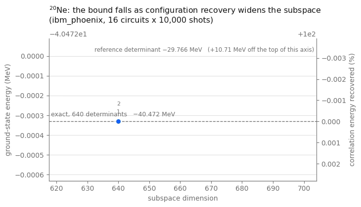
convergence_plot(
    result_sd["history"],
    E_REF_SD,
    E_EXACT_SD,
    f"$^{{20}}$Ne: the bound falls as configuration recovery widens the subspace\n"
    f"({backend.name}, {N_CIRCUITS} circuits x {SHOTS:,} shots)",
    full_dim=len(basis_exact_sd),
)
plt.show()
대규모 하드웨어 예제
규모를 키워도 바뀌는 것은 입력뿐이므로, 다음 단계에서는 네 단계를 하나의 함수로 묶어 두 번 실행합니다. 두 번 모두 GXPF1 상호작용 [3]을 사용하여 코어 위 껍질의 40큐비트 레지스터에서 실행합니다.
두 실행은 규모 확장의 서로 다른 측면을 보여 줍니다.
-
는 원자가 양성자 2개와 원자가 중성자 2개를 가지며 4,000개 행렬식의 기저를 가집니다. 레지스터는 40큐비트이지만 문제는 여전히 노트북에서 정확하게 대각화할 수 있을 만큼 작으므로, 레지스터 크기를 늘린 뒤에도 하드웨어 결과를 정확한 기준값과 비교할 수 있습니다.
-
는 원자가 양성자 4개와 원자가 중성자 4개를 가지며, 같은 40큐비트에서 대칭성이 허용하는 행렬식이 1,963,461개입니다. 이 튜토리얼의 밀집 솔버는 그 전체 공간을 대각화할 수 없으므로, 이 실행은 엄밀한 상한과 그 상한이 개선한 기준 행렬식을 반환합니다.
두 실행에 걸쳐 두 가지 양을 살펴보세요. 고정된 게이트 예산 안에 들어가는 풀의 비율은 풀이 커질수록 줄어들며, pack_ensemble이 얼마나 포함되었는지 보고합니다. 부분 공간은 샘플링이 아니라, 여기의 밀집 고전 솔버가 만들 수 있는 가장 큰 행렬인 MAX_DIMENSION에 의해 제한되기 시작합니다. 이 규모에서는 실제 운영 계산이라면 선택적 구성 상호작용(selected-CI) 솔버를 사용할 것입니다.
1–4단계 결합
다음 함수는 따라 하기에서와 같은 단계를 같은 순서로 호출합니다.
def sqd_run(snt_file, n_protons, n_neutrons, name, exact=True):
    """The whole workflow for one nucleus.  Returns a record of every stage."""
    # -------------------------Step 1-------------------------
    ms = read_snt(DATA / snt_file, n_protons, n_neutrons)
    sp = m_scheme_states(ms)
    inter = Interaction(ms, sp)
    if sum(1 for s in sp if s.tz == -1) * 2 != len(sp):
        raise ValueError(
            f"{name}: post-selection needs equal proton and neutron state counts"
        )
    reference = reference_determinant(sp, inter, n_protons, n_neutrons)
    e_ref = matrix_element(inter, reference, reference)

    raw = excitation_pool(sp, reference)
    ranked = rank_pool(
        inter, reference, [op for op in raw if conserves_symmetry(sp, op)]
    )
    print(
        f"{name}: {len(sp)} qubits, {n_protons}p + {n_neutrons}n, A = {ms.mass_number}"
    )
    print(
        f"  2p2h pool {len(raw)} raw -> {len(ranked)} symmetry-allowed; "
        f"reference energy {e_ref:.6f} MeV"
    )

    # -------------------------Step 2-------------------------
    costs = excitation_costs(len(sp), ranked, costing_manager)
    circuits, bins, isa = pack_to_budget(
        len(sp),
        reference,
        ranked,
        costs,
        DEPTH_BUDGET,
        N_CIRCUITS,
        pass_manager,
    )
    packed = sum(len(b) for b in bins)
    worst = max(two_qubit_depth(c) for c in isa)
    worst_count = max(two_qubit_count(c) for c in isa)
    print(
        f"  packed {packed} of {len(ranked)} excitations; worst circuit two-qubit depth "
        f"{worst}, {worst_count} two-qubit gates"
    )

    # -------------------------Step 3-------------------------
    # a unique tag per run, so the jobs are findable later
    bit_arrays = sample(isa, SHOTS, JOB_TAGS + [name])
    matrix, probabilities, shots = pool_samples(bit_arrays, sp)
    survival = float(
        probabilities[
            (matrix[:, len(sp) // 2 :].sum(axis=1) == n_protons)
            & (matrix[:, : len(sp) // 2].sum(axis=1) == n_neutrons)
        ].sum()
    )
    print(
        f"  {shots:,} shots -> {len(matrix):,} distinct bitstrings, "
        f"{survival:.1%} of shots with the right nucleon numbers"
    )
    if survival == 0.0:
        raise RuntimeError(
            f"{name}: no shot carried the right nucleon numbers"
        )

    # -------------------------Step 4-------------------------
    result = recovery_loop(
        inter,
        sp,
        matrix,
        probabilities,
        reference,
        n_protons,
        n_neutrons,
        max_iterations=4,
        max_dimension=MAX_DIMENSION,
        seed=42,
    )
    energy = result["energy"]

    full_dim = count_basis(sp, n_protons, n_neutrons)  # cheap, even when huge
    e_exact = None
    if exact:
        full = full_basis(sp, n_protons, n_neutrons)
        if len(full) != full_dim:
            raise AssertionError(
                f"{name}: counted {full_dim} determinants but enumerated "
                f"{len(full)}"
            )
        e_exact, _ = ground_state(inter, full)

    print(f"  reference {e_ref:11.6f} MeV     pooled SQD {energy:11.6f} MeV")
    if e_exact is not None:
        print(
            f"  exact     {e_exact:11.6f} MeV  (dimension {full_dim})  ->  "
            f"{100 * (energy - e_ref) / (e_exact - e_ref):.1f}% of the correlation energy"
        )
        if energy < e_exact - 1e-7:
            raise AssertionError(
                f"{name}: pooled SQD bound is below the exact energy"
            )
    else:
        print(
            f"  no exact reference: the symmetry-allowed basis is {full_dim:,} determinants"
        )
        print(
            f"  the bound captures {energy - e_ref:.6f} MeV of correlation energy"
        )
    print()

    return dict(
        name=name,
        qubits=len(sp),
        pool=len(ranked),
        packed=packed,
        two_qubit=worst,
        two_qubit_gates=worst_count,
        shots=shots,
        distinct=len(matrix),
        survival=survival,
        dimension=len(result["basis"]),
        full_dim=full_dim,
        e_ref=e_ref,
        e_sqd=energy,
        e_exact=e_exact,
        history=result["history"],
        # the subspace and its eigenvector cannot be reconstructed from the summary --
        # they depend on the sampled shots -- so keep them for the scaling analysis
        interaction=inter,
        states=sp,
        reference=reference,
        ranked=ranked,
        basis=result["basis"],
        vector=result["vector"],
    )

pretty = {"20Ne": "$^{20}$Ne", "44Ti": "$^{44}$Ti", "48Cr": "$^{48}$Cr"}

small_scale = dict(
    name="20Ne",
    qubits=len(sp_sd),
    pool=len(ranked_sd),
    packed=PACKED_SD,
    two_qubit=worst_sd,
    two_qubit_gates=worst_count_sd,
    shots=shots_sd,
    distinct=len(matrix_sd),
    survival=shot_survival_sd,
    dimension=len(result_sd["basis"]),
    full_dim=len(basis_exact_sd),
    e_ref=E_REF_SD,
    e_sqd=E_SQD_SD,
    e_exact=E_EXACT_SD,
    history=result_sd["history"],
    interaction=inter_sd,
    states=sp_sd,
    reference=occ_sd,
    ranked=ranked_sd,
    basis=result_sd["basis"],
    vector=result_sd["vector"],
)
: 40큐비트 레지스터에서의 같은 워크플로
위의 껍질은 종류당 네 개의 궤도와 각각 20개의 자기 부준위를 가지므로 레지스터는 40큐비트입니다. 원자가 양성자 2개와 원자가 중성자 2개가 를 이루며, 대칭성이 허용하는 행렬식은 4,000개로 기저의 약 6배이고, 24큐비트 대신 40큐비트를 사용합니다.
이것은 노트북이 정확하게 풀 수 있는 두 예제 중 더 큰 것이므로, 하드웨어 결과를 정확한 기준값과 비교할 수 있습니다.
large_scale_verified = sqd_run("gxpf1.snt", 2, 2, "44Ti", exact=True)
44Ti: 40 qubits, 2p + 2n, A = 44
  2p2h pool 1602 raw -> 174 symmetry-allowed; reference energy -44.309387 MeV
  packed 96 of 174 excitations; worst circuit two-qubit depth 272, 285 two-qubit gates
job dap31a02fm4c73f67dp0: 16 circuits x 10,000 shots on ibm_phoenix
  160,000 shots -> 48,170 distinct bitstrings, 18.6% of shots with the right nucleon numbers
  iteration 1: 187 proton x 189 neutron halves -> dimension 3891, E = -47.849086 MeV
  iteration 2: 190 proton x 190 neutron halves -> dimension 4000, E = -47.876666 MeV
  iteration 3: 190 proton x 190 neutron halves -> dimension 4000, E = -47.876666 MeV
  reference  -44.309387 MeV     pooled SQD  -47.876666 MeV
  exact      -47.876666 MeV  (dimension 4000)  ->  100.0% of the correlation energy
: 튜토리얼의 정확 대각화 용량을 넘어서
양성자 2개와 중성자 2개를 추가해도 같은 40큐비트 레지스터를 사용하며(의 경우 4, 4), 기저 크기는 약 491배 늘어 대칭성이 허용하는 행렬식 1,963,461개가 됩니다. 이 행렬은 이 튜토리얼이 만들 수 있는 범위를 훨씬 넘어서므로 exact=False입니다. 정확한 기준 에너지는 없고, 변분 한계와 그 한계가 개선한 기준 행렬식만 있습니다.
이 규모에서는 두 가지가 달라지며, 둘 다 출력 결과에서 확인할 수 있습니다. 풀(pool)이 수백 개의 허용된 들뜸(excitation)으로 커지므로, 고정된 게이트 예산은 이제 전체가 아니라 일부만 포괄합니다. 또한 샘플이 걸치는 곱 부분공간이 MAX_DIMENSION보다 크기 때문에, 밀집 솔버가 샘플링된 가중치 기준으로 이를 잘라 냅니다. 이 한계(bound)는 여전히 엄밀하지만, 샘플링된 모든 구성으로 계산한 한계보다 정확도가 낮을 수 있습니다. 실제 운영 환경의 계산에서는 샘플을 보존하고 더 큰 부분공간을 지원하는 솔버를 사용할 것입니다.
large_scale_unverified = sqd_run("gxpf1.snt", 4, 4, "48Cr", exact=False)
48Cr: 40 qubits, 4p + 4n, A = 48
  2p2h pool 5536 raw -> 582 symmetry-allowed; reference energy -93.041237 MeV
  packed 96 of 582 excitations; worst circuit two-qubit depth 224, 279 two-qubit gates
job dap32a02fm4c73f67eog: 16 circuits x 10,000 shots on ibm_phoenix
  160,000 shots -> 55,436 distinct bitstrings, 18.6% of shots with the right nucleon numbers
  iteration 1: 223 proton x 223 neutron halves -> dimension 3977, E = -96.481598 MeV
  iteration 2: 223 proton x 223 neutron halves -> dimension 3977, E = -96.481598 MeV
  reference  -93.041237 MeV     pooled SQD  -96.481598 MeV
  no exact reference: the symmetry-allowed basis is 1,963,461 determinants
  the bound captures -3.440361 MeV of correlation energy
정확한 기준 없이 결과 평가하기
실행에는 이 튜토리얼 안에서 정확한 기준값이 없습니다. 추가 QPU 시간이나 전체 공간 대각화 없이, 기존 샘플을 사용해 수렴 여부를 평가하고 고전적 선택 기준선과 비교합니다.
수렴했나요? 유지한 행렬식을 수렴된 고유벡터에서의 가중치 순으로 재정렬하면 부분공간이 중첩됩니다. 따라서 의 사다리(ladder)에 대해 선두 블록을 대각화하면, 부분공간 크기 두 자릿수에 걸친 한계의 하강 추이를 추적할 수 있습니다. 가장 큰 에서도 여전히 가파르게 떨어지고 있다면, 고전 솔버의 차원 상한이 결정적인 제약이며 MAX_DIMENSION이 늘려야 할 매개변수입니다. 곡선이 평평해졌다면, 유지한 행렬식을 더 추가해도 개선 효과가 거의 없습니다. 더 나아가려면 추가 구성을 샘플링해야 할 수 있습니다. 해밀토니안은 전체 크기로 한 번만 구성하고 각 단계는 그 주 블록(principal block)이므로, 전체 스윕에 필요한 행렬 구성은 단계마다가 아니라 한 번뿐입니다.
양자 샘플링은 고전적 선택과 어떻게 비교될까요? 고전적 선택 절차로 고른 같은 크기의 부분공간과 비교합니다. 섭동 이론 점수 순서로 정렬한 풀에서 같은 차원이 될 때까지 곱 부분공간을 키운 뒤 그것을 대신 대각화합니다. 두 곡선 모두 같은 해밀토니안에 대한 엄밀한 상한이므로, 같은 차원에서 더 낮은 쪽이 더 좋은 행렬식을 골랐다는 뜻입니다. 이 비교는 하드웨어 샘플링이 이 고전적 기준선 대비 에너지 추정을 개선하는지 판단해 줍니다.
이 부분공간은 들뜬 상태를 위해 선택된 것이 아닙니다. 구성 복구(configuration recovery)는 바닥 상태 점유율을 사용해 부분공간을 유도하므로, 더 높은 고윳값은 가장 낮은 고윳값보다 수렴과 훨씬 거리가 멀고, 첫 번째 들뜸 에너지는 측정된 보다 훨씬 높게 나옵니다. 들뜬 상태에 제대로 도달하려면 그것을 위해 선택된 부분공간이 필요합니다.
def subspace_scaling(
    inter, basis, vector, points=18, smallest=32, largest=None
):
    """Nested Rayleigh-Ritz sweep: the lowest eigenvalue of the leading d x d block, for a ladder of d.

    Reordering the basis by descending weight in the converged eigenvector makes every subspace in
    the ladder a subset of the next, so the energies fall monotonically and each one is a valid
    variational bound.  H is built once at full size; each rung is a principal block.
    """
    order = np.argsort(-(np.abs(vector) ** 2))
    ordered = [basis[i] for i in order]
    weights = (np.abs(vector) ** 2)[order]
    if (
        largest is not None
    ):  # cap the ladder so two subspaces end at a common dimension
        ordered, weights = ordered[:largest], weights[:largest]
    H = subspace_hamiltonian(inter, ordered)
    dimensions = np.unique(
        np.geomspace(smallest, len(ordered), points).astype(int)
    )
    rows = [
        (
            int(d),
            float(
                eigh(H[:d, :d], eigvals_only=True, subset_by_index=[0, 0])[0]
            ),
        )
        for d in dimensions
    ]
    return rows, np.cumsum(weights)

def classical_selection(
    inter, sp, reference, ranked, target, n_protons, n_neutrons
):
    """The subspace classical perturbative ranking would pick, grown to `target` dimension.

    Same product construction as the sampled subspace, and the same truncation discipline -- half
    configurations are offered to `grow_subspace` in order of importance and it takes as many as
    fit.  The only difference from the sampled path is where the ordering comes from: PT2 score
    here, measured sampling weight there.  So the comparison isolates *which determinants got
    chosen* and nothing else.

    Truncating by any other rule would not be a fair baseline.  Slicing an arbitrarily ordered
    list, for instance, keeps determinants by accident rather than by importance and makes the
    classical subspace look worse than classical selection really is.
    """
    p_ref = tuple(i for i in reference if sp[i].tz == -1)
    n_ref = tuple(i for i in reference if sp[i].tz == +1)
    reached = {reference}
    proton_order, neutron_order = [p_ref], [n_ref]
    seen_p, seen_n = {p_ref}, {n_ref}
    product_budget = 4 * target

    for op, _, _ in ranked:  # ranked is already in descending PT2 score
        h1, h2, v1, v2 = op
        fresh = {
            tuple(sorted(set(d) - {h1, h2} | {v1, v2}))
            for d in reached
            if {h1, h2} <= set(d) and not {v1, v2} & set(d)
        }
        reached |= fresh
        for det in fresh:  # first appearance fixes a half's rank
            half_p = tuple(i for i in det if sp[i].tz == -1)
            half_n = tuple(i for i in det if sp[i].tz == +1)
            if half_p not in seen_p:
                seen_p.add(half_p)
                proton_order.append(half_p)
            if half_n not in seen_n:
                seen_n.add(half_n)
                neutron_order.append(half_n)
        if len(proton_order) * len(neutron_order) > product_budget:
            # Half-configuration products over-count the subspace, because only the
            # symmetry-allowed ones survive `product_subspace`.  Stopping on the product
            # count alone can therefore leave the basis far short of `target`, so check
            # the dimension actually realized and widen the budget if it falls short.
            trial, _, _ = grow_subspace(
                sp,
                [p_ref],
                [n_ref],
                proton_order,
                neutron_order,
                n_protons,
                n_neutrons,
                max_dimension=target,
            )
            if len(trial) >= target:
                break
            product_budget *= 2

    basis, _, _ = grow_subspace(
        sp,
        [p_ref],
        [n_ref],
        proton_order,
        neutron_order,
        n_protons,
        n_neutrons,
        max_dimension=target,
    )
    return basis

run = large_scale_unverified
if "basis" not in run:
    raise RuntimeError(
        "this cell needs the subspace and eigenvector that sqd_run now returns; "
        "re-run the sqd_run definition and the 48Cr cell"
    )

print(
    f"{run['name']}: sweeping nested subspaces of the sampled basis "
    f"(dimension {run['dimension']})"
)
sampled_rows, cumulative = subspace_scaling(
    run["interaction"], run["basis"], run["vector"]
)

print(
    f"{run['name']}: building the classically selected subspace at the same dimension"
)
classical_basis = classical_selection(
    run["interaction"],
    run["states"],
    run["reference"],
    run["ranked"],
    run["dimension"],
    4,
    4,
)
# Both subspaces must be scored at the same dimension.  Symmetry filtering can still leave
# the classical construction short of the target when the ranked pool runs out, so take the
# dimension both actually reach, cap both ladders there, and verify they agree.
common_dim = min(sampled_rows[-1][0], len(classical_basis))
if common_dim < sampled_rows[-1][0]:
    sampled_rows, _ = subspace_scaling(
        run["interaction"], run["basis"], run["vector"], largest=common_dim
    )
classical_rows, _ = subspace_scaling(
    run["interaction"],
    classical_basis,
    ground_state(run["interaction"], classical_basis)[1],
    largest=common_dim,
)
if sampled_rows[-1][0] != classical_rows[-1][0]:
    raise RuntimeError(
        f"comparison dimensions differ: sampled {sampled_rows[-1][0]}, "
        f"classical {classical_rows[-1][0]}"
    )

advantage = sampled_rows[-1][1] - classical_rows[-1][1]
direction = "lower" if advantage < 0 else "higher"
verdict = "beats" if advantage < 0 else "does not beat"
descent = next(
    e for d, e in reversed(sampled_rows) if d <= sampled_rows[-1][0] / 2
)
for fraction in (0.90, 0.99):
    count = int(np.searchsorted(cumulative, fraction) + 1)
    print(
        f"  {fraction:.0%} of the eigenvector norm sits on {count} determinants "
        f"({count / run['full_dim']:.1e} of the {run['full_dim']:,}-determinant space)"
    )
print(
    f"  bound still falling {1000 * (sampled_rows[-1][1] - descent):+.1f} keV "
    f"over the last doubling of dimension"
)
print(
    f"  sampled {sampled_rows[-1][1]:.6f} MeV vs classically selected "
    f"{classical_rows[-1][1]:.6f} MeV at a verified common dimension of "
    f"{classical_rows[-1][0]:,}"
)
print(
    f"  -> the sampled subspace is {abs(advantage) * 1000:.0f} keV {direction}"
)
48Cr: sweeping nested subspaces of the sampled basis (dimension 3977)
48Cr: building the classically selected subspace at the same dimension
  90% of the eigenvector norm sits on 107 determinants (5.4e-05 of the 1,963,461-determinant space)
  99% of the eigenvector norm sits on 593 determinants (3.0e-04 of the 1,963,461-determinant space)
  bound still falling -15.6 keV over the last doubling of dimension
  sampled -96.481598 MeV vs classically selected -95.314510 MeV at a verified common dimension of 3,957
  -> the sampled subspace is 1167 keV lower
fig, axes = plt.subplots(1, 2, figsize=(11.2, 4.0), facecolor=SURFACE)

# left: two nested convergence curves on the same axes
ax = axes[0]
ax.set_facecolor(SURFACE)
ax.plot(
    [d for d, _ in sampled_rows],
    [e for _, e in sampled_rows],
    "-o",
    color=SERIES,
    linewidth=2,
    markersize=5,
    markeredgecolor=SURFACE,
    markeredgewidth=1,
    zorder=4,
    label="sampled on the QPU",
)
ax.plot(
    [d for d, _ in classical_rows],
    [e for _, e in classical_rows],
    "--s",
    color=MUTED,
    linewidth=1.6,
    markersize=4,
    markeredgecolor=SURFACE,
    markeredgewidth=1,
    zorder=3,
    label="classically selected, same size",
)
ax.axhline(run["e_ref"], color=RULE, linestyle=":", linewidth=1.2, zorder=1)
ax.annotate(
    f"reference determinant {run['e_ref']:.2f} MeV".replace("-", "\u2212"),
    xy=(sampled_rows[-1][0], run["e_ref"]),
    xytext=(-2, 4),
    textcoords="offset points",
    ha="right",
    va="bottom",
    color=MUTED,
    fontsize=8,
)

# mark the gap between the two curves at the largest dimension, not either curve alone
edge = sampled_rows[-1][0]
ax.plot(
    [edge, edge],
    [classical_rows[-1][1], sampled_rows[-1][1]],
    "-",
    color=SERIES,
    linewidth=1.0,
    alpha=0.7,
    zorder=2,
)
ax.annotate(
    f"{abs(advantage) * 1000:.0f} keV {direction}\nat equal dimension",
    xy=(edge, 0.5 * (classical_rows[-1][1] + sampled_rows[-1][1])),
    xytext=(-8, 0),
    textcoords="offset points",
    ha="right",
    va="center",
    color=SERIES,
    fontsize=8.5,
)

ax.set_xscale("log")
ax.set_xlim(sampled_rows[0][0] * 0.75, edge * 1.5)
ax.set_xlabel("subspace dimension", color=MUTED)
ax.set_ylabel("variational upper bound (MeV)", color=MUTED)
ax.set_title(
    f"{pretty[run['name']]}: the bound, and the subspace it {verdict}",
    color=INK,
    fontsize=11,
    loc="left",
    pad=10,
)
legend = ax.legend(frameon=False, fontsize=8.5, loc="lower left")
for text in legend.get_texts():
    text.set_color(MUTED)

# right: why a few thousand determinants can bound two million
ax = axes[1]
ax.set_facecolor(SURFACE)
ranks = np.arange(1, len(cumulative) + 1)
ax.plot(ranks, 100 * cumulative, "-", color=DEEP, linewidth=2, zorder=3)
for fraction, style, label_y in ((0.90, ":", 46), (0.99, "--", 24)):
    count = int(np.searchsorted(cumulative, fraction) + 1)
    ax.axvline(count, color=MUTED, linestyle=style, linewidth=1, zorder=1)
    ax.annotate(
        f"{fraction:.0%} of the norm\non {count} determinants",
        xy=(count, label_y),
        xytext=(7, 0),
        textcoords="offset points",
        ha="left",
        va="center",
        color=MUTED,
        fontsize=8.5,
    )
ax.set_xscale("log")
ax.set_xlim(0.8, len(cumulative) * 2.6)
ax.set_ylim(0, 104)
ax.set_xlabel("determinants, ordered by weight", color=MUTED)
ax.set_ylabel("cumulative share of the eigenvector (%)", color=MUTED)
ax.set_title(
    f"Sparsity: {run['full_dim']:,} determinants in the sector",
    color=INK,
    fontsize=11,
    loc="left",
    pad=10,
)

for ax in axes:
    ax.grid(axis="y", color=RULE, alpha=0.55)
    ax.tick_params(colors=MUTED, labelsize=8.5)
    for side in ("top", "right"):
        ax.spines[side].set_visible(False)
    for side in ("bottom", "left"):
        ax.spines[side].set_color(MUTED)
fig.tight_layout()
plt.show()
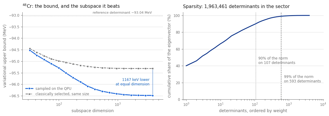
세 번의 실행 비교하기
절대 에너지는 서로 다른 핵과 서로 다른 상호작용 사이에서 비교할 수 없으므로, 정확한 기준값을 구할 수 있는 경우 각 실행에서 복구된 상관 에너지의 비율에 주목합니다. 회로 깊이와 폐기된 샷의 비율도 함께 비교합니다.
runs = [small_scale, large_scale_verified, large_scale_unverified]

print(
    f"{'run':>6}  {'qubits':>6}  {'pool':>9}  {'2q depth':>8}  {'2q gates':>8}  "
    f"{'shots kept':>10}  {'dim':>6}  {'of':>9}  {'% corr':>7}"
)
for r in runs:
    fraction = (
        "--"
        if r["e_exact"] is None
        else f"{100 * (r['e_sqd'] - r['e_ref']) / (r['e_exact'] - r['e_ref']):.1f}%"
    )
    coverage = "{}/{}".format(r["packed"], r["pool"])
    print(
        f"{r['name']:>6}  {r['qubits']:>6}  {coverage:>9}  "
        f"{r['two_qubit']:>8}  {r['two_qubit_gates']:>8}  {r['survival']:>9.1%}  "
        f"{r['dimension']:>6}  {(r['full_dim'] or 0):>9,}  {fraction:>7}"
    )

print()
for r in runs:
    exact = (
        f"exact {r['e_exact']:11.6f}"
        if r["e_exact"] is not None
        else "exact  unavailable"
    )
    print(
        f"{r['name']:>6}   reference {r['e_ref']:11.6f}   pooled SQD {r['e_sqd']:11.6f}   {exact} MeV"
    )
run  qubits       pool  2q depth  2q gates  shots kept     dim         of   % corr
  20Ne      24      78/78       228       234      31.5%     640        640   100.0%
  44Ti      40     96/174       272       285      18.6%    4000      4,000   100.0%
  48Cr      40     96/582       224       279      18.6%    3977  1,963,461       --

  20Ne   reference  -29.765549   pooled SQD  -40.472331   exact  -40.472331 MeV
  44Ti   reference  -44.309387   pooled SQD  -47.876666   exact  -47.876666 MeV
  48Cr   reference  -93.041237   pooled SQD  -96.481598   exact  unavailable MeV
# Left: how much of the correlation energy was recovered, where the exact answer is known.
# Right: the bound itself for the run that has nothing to score against.
scored = [r for r in runs if r["e_exact"] is not None]

fig, ax = plt.subplots(figsize=(6.4, 3.9), facecolor=SURFACE)
ax.set_facecolor(SURFACE)
labels = [
    f"{pretty[r['name']]}\n{r['qubits']} qubits\n{r['full_dim']:,} determinants"
    for r in scored
]
fractions = [
    100 * (r["e_sqd"] - r["e_ref"]) / (r["e_exact"] - r["e_ref"])
    for r in scored
]
shades = [SERIES, DEEP, PURPLE]
bars = ax.bar(
    labels, fractions, width=0.46, color=shades[: len(scored)], zorder=3
)
for bar, fraction, r in zip(bars, fractions, scored):
    ax.annotate(
        f"{fraction:.1f}%",
        xy=(bar.get_x() + bar.get_width() / 2, fraction),
        xytext=(0, 5),
        textcoords="offset points",
        ha="center",
        va="bottom",
        color=INK,
        fontsize=10,
    )
    ax.annotate(
        f"dim {r['dimension']:,}",
        xy=(bar.get_x() + bar.get_width() / 2, 3),
        ha="center",
        va="bottom",
        color=SURFACE,
        fontsize=8.5,
    )
ax.axhline(100, color=MUTED, linestyle="--", linewidth=1, zorder=1)
ax.annotate(
    "exact diagonalization",
    xy=(-0.45, 100),
    xytext=(0, 4),
    textcoords="offset points",
    ha="left",
    va="bottom",
    color=MUTED,
    fontsize=8.5,
)
ax.set_ylim(0, 118)
ax.set_ylabel("correlation energy recovered (%)", color=MUTED)
ax.set_title(
    f"Where the exact answer is known ({backend.name})",
    color=INK,
    fontsize=11,
    loc="left",
    pad=10,
)
ax.grid(axis="y", color=RULE, alpha=0.55)
ax.tick_params(colors=MUTED, labelsize=8.5)
for side in ("top", "right"):
    ax.spines[side].set_visible(False)
for side in ("bottom", "left"):
    ax.spines[side].set_color(MUTED)
fig.tight_layout()
plt.show()

# the same convergence view as the walkthrough, for the run with no exact reference
convergence_plot(
    large_scale_unverified["history"],
    large_scale_unverified["e_ref"],
    None,
    f"{pretty[large_scale_unverified['name']]}: "
    f"{large_scale_unverified['full_dim']:,} determinants, no exact answer to score against\n"
    f"({backend.name}, {N_CIRCUITS} circuits x {SHOTS:,} shots)",
    colour=DEEP,
)
plt.show()

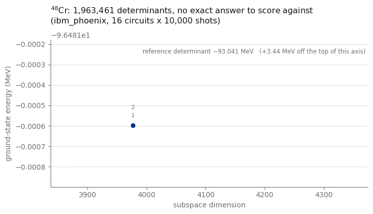
요약
입력만 바꾸고 나머지는 그대로인 하나의 워크플로를 세 가지 문제 크기로 QPU에서 실행했습니다. 정확히 검증할 수 있는 24큐비트 문제, 여전히 정확히 검증할 수 있는 40큐비트 문제, 그리고 이 튜토리얼의 정확한 대각화 능력을 넘어서는 약 200만 개의 기저 상태를 가진 40큐비트 문제입니다.
세 번의 실행은 다음 점들을 보여 줍니다.
-
양자 단계는 행렬식을 제안하기만 하면 됩니다. 회로는 고정되어 있고, 2차 섭동 이론으로 시드되며, 최적화되지 않습니다. 워크플로에서 진폭이 정확해야 할 필요는 전혀 없고, 그 지지집합(support)이 유용하기만 하면 됩니다. 선택된 부분공간에서의 고전 대각화는 변분 상한을 제공하지만, 이 한계는 샘플링된 구성에 따라 달라집니다.
-
큐비트 들뜸은 회로 깊이를 줄입니다. 중요한 것은 지지집합뿐이므로, 페르미온 들뜸 블록을 큐비트 들뜸으로 대체할 수 있고, 그 비용은 연결하는 오비탈 사이의 거리에 따라 늘어나지 않습니다. 2단계에서 실제 백엔드에서 절감 효과를 측정했으며, 이는 결맞음 시간 안에 여유 있게 들어가는 회로와 그렇지 않은 회로의 차이입니다.
-
구성 복구는 잡음이 있는 샘플을 재활용합니다. 양성자 또는 중성자 수가 잘못된 모든 샷은 폐기되지 않고 현재 점유율 추정에 맞춰 복구되며, 복구된 각 반쪽 구성은 부분공간에 구성을 추가할 수 있습니다. 변분 부분공간을 넓혀도 그 최저 고윳값은 올라갈 수 없습니다. 이 튜토리얼은 하드웨어 샘플을 사용한 구성 복구를 보여 줍니다.
-
규모를 키울수록 결정적 제약이 바뀝니다. 24큐비트에서는 앤사츠가 정확한 답에 도달할 수 있었고, 샘플링만이 걸림돌이었습니다. 종(species)당 원자가 핵자가 4개인 40큐비트에서는 게이트 예산이 풀의 일부만 포괄하고 밀집 고전 솔버가 부분공간을 제한합니다. 세 가지 중 무엇이 한계로 작용하는지 아는 것이 이 워크플로가 가르치는 실용적인 기술입니다.
다음 단계
다음 관련 자료를 살펴보세요.
-
화학 해밀토니안의 샘플 기반 양자 대각화: SQD 애드온의 selected-CI 솔버를 사용해 전자 구조에 같은 알고리즘을 적용합니다.
-
SQD 애드온 문서: 사후 선택(post-selection), 서브샘플링, 구성 복구 유틸리티를 다룹니다.
-
양자 대각화 알고리즘: Krylov 변형을 포함한 부분공간 대각화 전체 과정입니다.
-
트랜스파일 소개: 회로에서 2큐비트 게이트가 지배적일 때 중요한 패스 매니저 옵션을 설명합니다.
-
실행 모드: 독립적인 작업을 스케줄링하는 batch mode를 살펴봅니다.
고려해 볼 확장
-
밀집 솔버 교체하기. 규모에서는
MAX_DIMENSION이 모든 것의 상한이며, 그 이유는 밀집 행렬에 대한np.linalg.eigh입니다. 같은 사영 해밀토니안을 희소 행렬로 구성하고scipy.sparse.linalg.eigsh같은 반복 고유값 솔버, 또는 핵의 2체 상호작용을 위해 설계된 Davidson 또는 selected-CI 솔버를 사용하면 더 큰 부분공간을 지원할 수 있습니다. 실제 한계는 행렬의 희소성, 사용 가능한 메모리, 솔버 수렴에 따라 달라지며, 이 튜토리얼은 이 확장을 벤치마크하지 않습니다. SQD 애드온의qiskit_addon_sqd.fermion.solve_sci는 그대로 대체할 수 없습니다. 이 함수는 전자 구조 솔버를 감싸고 있으며 그 형태의 1체 및 2체 적분을 요구하므로, 공유된 양성자 중성자 곱 구조만으로는 충분하지 않습니다. 이를 사용하려면 식 (1)의 껍질 모형 상호작용을 그 적분으로 매핑하고, 이 노트북이 이미 계산한 정확한 에너지와 결과를 대조해 검증해야 합니다. -
배칭과 서브샘플링 추가하기. 발표된 풀링 SQD 워크플로는 반복마다 여러 독립 서브샘플을 대각화하고 가장 좋은 것을 유지합니다. 이 튜토리얼은 반복마다 하나의 배치를 사용하는데, 변분 한계에는 해가 없지만 샷을 더 늘리는 것이 도움이 될지 알려 주는 분산 정보는 제공하지 못합니다.
-
들뜬 상태와 다른 섹터. 각 부분공간 해밀토니안의 더 높은 고윳값은 같은 대칭 섹터에 있는 들뜬 상태의 상한이며, 에서 실행하면 다른 섹터에 도달합니다. 1단계의 확인은 이미 이 계산의 절반입니다.
-
껍질 간 모형 공간. 단일 주 껍질 안에서는 홀짝성(parity)이 자동으로 만족되므로 여기서는 아무 역할도 하지 않습니다. - 공간은 홀짝성을 섞어 홀짝성을 진정한 네 번째 제약으로 만들며, 이는 SQD의 해밍 가중치 복구도 곱 구성도 스스로는 잡아내지 못하는 제약입니다.
-
홀수 질량 핵.
reference_determinant는 각 종의 원자가 개수가 짝수여야 하는데, 시간 반전 쌍으로 채우는 것이 을 강제하기 때문입니다. 홀수 핵에는 반정수 목표와 짝지어지지 않은 기준이 필요합니다.
부록
이 절에서는 설정 절에서 소개한 헬퍼 함수들의 배경 논리를 설명합니다.
질량 의존 재조정이 선택 사항이 아닌 이유
경험적 껍질 모형 상호작용은 하나의 질량에서 피팅되어 동위원소 사슬 전체에 적용되며, 2체 행렬 요소는 로 조정됩니다. 두 상호작용 파일 모두 을 가지며, 는 USD 계열에서 , GXPF1에서 입니다. .snt 파일의 2체 헤더 줄에서 이 두 숫자는 진동수와 코어 에너지가 들어갈 법한 자리에 놓여 있어 잘못 읽기 쉽습니다. 지수를 상수 코어 에너지로 읽으면 모든 대각 요소에 허위 오프셋이 더해지고 동시에 재조정이 빠져서 상관 에너지가 몇 퍼센트 달라집니다. 1단계의 대칭 확인만으로는 에너지 척도를 검증하지 못합니다. MeV 단위로 측정한 들뜸 에너지를 실험값과 비교하면 질량 의존 재조정에 대한 추가 확인이 됩니다. 들뜸 에너지는 준위 사이의 차이이므로 모든 에너지에 적용된 상수 오프셋은 감지하지 못합니다.
기준을 채우기가 아니라 탐색으로 찾는 이유
가장 명백한 기준은 가장 낮은 단일 입자 에너지를 채우는 행렬식입니다. 하지만 이것이 가장 낮은 에너지의 행렬식은 아닙니다. 식 (1)의 대각 성분에 2체 항 가 포함되고, 쌍 상호작용은 사용 가능한 가장 큰 에 시간 반전 짝을 채우는 쪽을 강하게 선호하기 때문입니다. 껍질에서 이는 쌍과 의 쌍의 차이이며 약 1 MeV에 해당합니다. 껍질에서는 2 MeV에 가깝습니다. 기준 에너지가 "복구된 상관 에너지" 지표의 영점을 정하므로, 나쁜 선택은 그 지표를 부풀리고 덜 정확한 출발점을 제공합니다.
짝지은 채우기로 제한하면 종마다 개(많아야 수천 개)의 후보만 있어 전수 탐색이 저렴해지고 이 보장됩니다. 이 튜토리얼에서 전체 열거와 대조할 수 있는 모든 경우에, 탐색은 전역 최저 대각 성분의 행렬식을 반환하며, 이는 정확한 바닥 상태의 가장 큰 단일 성분이기도 합니다.
정확한 2준위 각도가 아니라 1차 진폭을 쓰는 이유
공간 에서 해밀토니안을 대각화하면 혼합각 가 나오며, 고립된 한 쌍의 준위에는 이것이 올바른 선택이라고 부르고 싶어질 수 있습니다. 이 앤사츠에서는 수십 개의 들뜸 블록이 같은 기준 위에서 차례로 작용하므로, 각 블록을 따로 최적화한다고 해서 합성 회로가 반드시 최적화되는 것은 아닙니다.
각도의 선택은 회로의 역할에 따라 결정됩니다. 모든 실수 에 대해 이므로, 정확한 각도는 항상 1차 진폭 보다 크기가 작고, 따라서 항상 기준 행렬식에 더 많은 진폭을 남깁니다. 기준에 더 많은 진폭을 남기는 회로는 기준을 더 자주 반환하고 서로 다른 들뜬 행렬식은 덜 자주 반환합니다. 풀링 SQD에서 샷의 유용한 출력은 고전 단계가 아직 보지 못한 행렬식이므로, 이 튜토리얼에서 더 큰 각도를 쓰는 동기가 됩니다. 고전 대각화가 회로의 진폭을 완전히 버리고 자체 진폭을 다시 구하므로, 어느 각도도 정확할 필요는 없습니다.
풀링 SQD가 큐비트 들뜸을 쓸 수 있는 이유
페르미온 들뜸 은 Jordan-Wigner 변환으로 8개의 파울리 문자열에 대응되며, 각 문자열은 가장 바깥쪽 인덱스 사이의 모든 큐비트에 연산자를 가집니다. 이 문자열들은 페르미온 부호를 인코딩하며 그 비용은 범위(span)에 따라 늘어나는데, 양성자-중성자 들뜸의 경우 범위가 레지스터 전체입니다.
이를 제거하면 Yordanov 등의 큐비트 들뜸 연산자 [5]가 됩니다. 이것은 다른 연산자입니다. 준비되는 상태는 진폭의 부호에서 페르미온 상태와 다르고, 두 샘플링 분포는 크게 다를 수 있습니다. 바뀌지 않는 것은 어떤 행렬식이 0이 아닌 진폭을 갖는지입니다. 각 블록은 작용하는 모든 행렬식 에 대해 여전히 같은 2차원 공간 안에서 회전하고, 두 핵자 수, , 홀짝성을 여전히 정확히 보존하기 때문입니다. 따라서 도달 가능한 행렬식 집합은 동일하며, 풀링 SQD가 사용하는 것은 이 도달 가능 집합뿐입니다. 고전 대각화는 어쨌든 자체 진폭을 부여합니다. 2단계에서는 풀의 실제 연산자로 동일 지지집합 주장을 검증하고, 이 대체로 얼마나 절감되는지 측정합니다.
한계는 샘플링 가중치가 다르다는 점이며, 따라서 두 구성은 유한한 샷 수에서 같은 순서로 행렬식을 발견하지 않습니다. 어떤 들뜸이 회로에 들어갈지 정하는 순위는 고전적이고 변하지 않으며 고전 단계가 어차피 모든 것을 다시 가중하므로, 샘플링 가중치의 차이는 회로 깊이 감소를 위한 절충입니다.
가 곱 단계에 속하는 이유
사후 선택과 구성 복구는 모두 해밍 가중치에 작용합니다. 즉 레지스터 한쪽 절반의 양성자 수와 다른 절반의 중성자 수입니다. 은 그런 형태가 아닙니다. 이는 양성자 구성이 중성자 구성과 짝지어졌을 때의 성질입니다. 양성자 절반과 중성자 절반이 각각 올바른 핵자 수를 가진 샷은, 값이 상쇄되지 않더라도 사용 가능한 반쪽 구성을 둘 포함합니다. 인 양성자 절반은 인 중성자 절반과 짝지어지면 완벽히 좋기 때문입니다. 전체 로 샷 전체를 거르면 두 절반이 모두 버려지고, 재결합한 곱에 를 부과하면 둘 다 유지됩니다. 같은 논리로 이 경우 recover_configurations가 유용하기 위해 개념이 필요 없는 이유도 설명됩니다.
참고 문헌
-
J. Robledo-Moreno, M. Motta, H. Haas, et al., "Chemistry beyond the scale of exact diagonalization on a quantum-centric supercomputer", Science Advances 11, eadu9991 (2025). arXiv:2405.05068
-
B. A. Brown and W. A. Richter, "New USD Hamiltonians for the sd shell", Physical Review C 74, 034315 (2006). The embedded
usda.sntfile carries the USDA parameters as tabulated by W. A. Richter, S. Mkhize and B. A. Brown, "sd-shell observables for the USDA and USDB Hamiltonians", Physical Review C 78, 064302 (2008). -
M. Honma, T. Otsuka, B. A. Brown and T. Mizusaki, "Effective interaction for pf-shell nuclei", Physical Review C 65, 061301(R) (2002).
-
B. Huron, J. P. Malrieu and P. Rancurel, "Iterative perturbation calculations of ground and excited state energies from multiconfigurational zeroth-order wavefunctions", The Journal of Chemical Physics 58, 5745 (1973).
-
Y. S. Yordanov, D. R. M. Arvidsson-Shukur and C. H. W. Barnes, "Efficient quantum circuits for quantum computational chemistry", Physical Review A 102, 062612 (2020).
-
National Nuclear Data Center, Evaluated Nuclear Structure Data File, Brookhaven National Laboratory. 1단계에서 인용한 측정된 들뜸 에너지의 출처입니다.