빠른 시작

이 가이드는 qiskit-addon-obp 패키지의 최소 작동 예제를 보여 줍니다. 연산자 역전파(OBP)를 사용하여 뒤쪽 게이트를 관측량에 흡수시킴으로써 양자 회로의 깊이를 줄입니다.

기댓값 $\langle O \rangle = \langle \psi | U^\dagger O U | \psi \rangle$은 회로 $U$의 뒤쪽 게이트 블록을 떼어 내어 관측량을 그 블록으로 고전적으로 켤레 변환해도 변하지 않습니다. OBP는 이를 반복해서 적용하여 회로의 일부를 고전적으로 평가하고, 더 얕은 회로만 하드웨어에서 실행되게 합니다. 대신 흡수된 게이트마다 관측량이 더 많은 Pauli 항으로 확장될 수 있으므로, 절약한 깊이와 관측량의 증가를 함께 따져 보아야 합니다.

이 도구로 현실적인 워크플로를 구성하고 양자 하드웨어에서 실행하는 예제를 보려면 IBM Quantum Platform의 튜토리얼(OBP Tutorial)을 확인하세요.

OBP 입력 준비하기

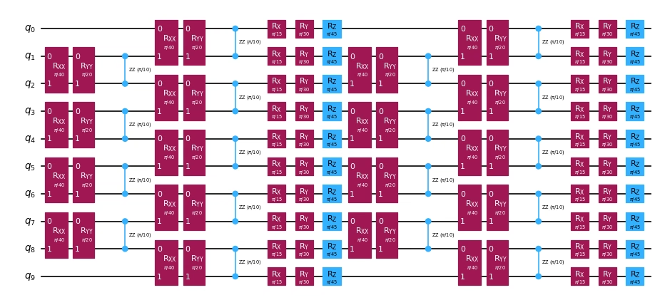
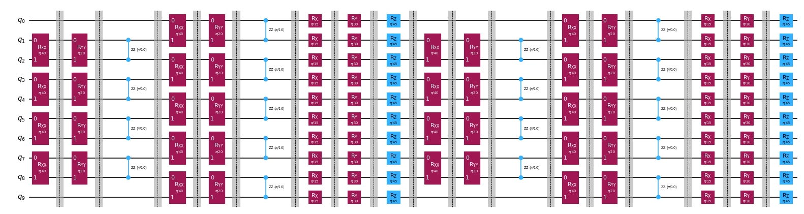
OBP는 회로 슬라이스 목록과 관측량을 입력으로 받습니다. 회로의 끝에서부터 슬라이스를 하나씩 관측량으로 역전파하며, 관측량의 Pauli 항이 늘어나는 대가로 회로 깊이를 줄입니다. 여기서는 10-큐비트 Heisenberg 모델의 시간 발전 회로를 생성하고 게이트 유형별로 슬라이스합니다.

아래에서는 원래 회로를 그린 다음, 슬라이스 경계를 배리어로 표시하여 다시 결합한 같은 회로를 그립니다. 각 슬라이스는 한 번의 역전파 단계로 관측량에 흡수될 수 있는 단위입니다.

# Added by doQumentation — installs the packages this notebook needs if they are missing
import importlib.util

_needed = {"numpy": "numpy", "qiskit": "qiskit", "qiskit_addon_obp": "qiskit-addon-obp", "qiskit_addon_utils": "qiskit-addon-utils"}
_missing = [pip for module, pip in _needed.items()
            if importlib.util.find_spec(module) is None]
# One at a time, so a package that fails to install does not block the others
for _pip in _missing:
    %pip install -q {_pip}
if not _missing:
    print("\u2713 All required packages are installed")

import numpy as np
from qiskit.quantum_info import SparsePauliOp
from qiskit.synthesis import LieTrotter
from qiskit.transpiler import CouplingMap
from qiskit_addon_utils.problem_generators import (
    generate_time_evolution_circuit,
    generate_xyz_hamiltonian,
)
from qiskit_addon_utils.slicing import combine_slices, slice_by_gate_types

# Generate a circuit to reduce
coupling_map = CouplingMap.from_heavy_hex(3, bidirectional=False)
reduced_coupling_map = coupling_map.reduce(
    [0, 13, 1, 14, 10, 16, 5, 12, 8, 18]
)

hamiltonian = generate_xyz_hamiltonian(
    reduced_coupling_map,
    coupling_constants=(np.pi / 8, np.pi / 4, np.pi / 2),
    ext_magnetic_field=(np.pi / 3, np.pi / 6, np.pi / 9),
)

circuit = generate_time_evolution_circuit(
    hamiltonian,
    time=0.2,
    synthesis=LieTrotter(reps=2),
)

# Slice the circuit and define an observable
slices = slice_by_gate_types(circuit)
observable = SparsePauliOp("IIIIIIIIIZ")

print(f"Original circuit depth: {circuit.depth()}")
print(f"Number of slices: {len(slices)}")
print(f"Observable terms: {len(observable)}")

Original circuit depth: 18
Number of slices: 18
Observable terms: 1

# Recombine the slices with barriers to make the slice boundaries visible
sliced_circuit = combine_slices(slices, include_barriers=True)

print("Original circuit:")
display(circuit.draw("mpl", scale=0.6, fold=-1))
print("Sliced circuit (recombined with barriers for visualization)")
sliced_circuit.draw("mpl", scale=0.6, fold=-1)

Original circuit:

Sliced circuit (recombined with barriers for visualization)

OBP로 회로 깊이 줄이기

backpropagate를 호출하여 슬라이스를 관측량에 흡수시킵니다. 이 함수는 확장된 관측량, 역전파되지 않은 회로 슬라이스, 그리고 과정에 대한 메타데이터를 반환합니다.

제한하지 않으면 관측량은 $2^n$개의 Pauli 항까지 늘어날 수 있습니다. operator_budget이 이 증가를 제한합니다. 여기서는 최대 8개의 큐비트별 가환 그룹을 허용하며, 이는 QPU에서 관측량을 평가하는 데 필요한 샷 수를 대략 결정합니다. 다음 슬라이스를 흡수하면 예산을 초과하게 되는 즉시 역전파가 중단되며, 아래에서 바로 그런 일이 일어납니다. 관측량이 가환 그룹 8개를 모두 채우기 전까지 18개 슬라이스 중 7개만 흡수되고 절차가 멈춥니다.

회로의 더 깊은 곳까지 나아가려면 backpropagate의 truncation_error_budget 키워드 인수를 사용하여 관측량이 커지는 동안 계수가 작은 Pauli 항을 버릴 수 있습니다. 이렇게 하면 절단되는 Pauli 항의 크기에 비례하는 약간의 오차를 감수하는 대신 관측량의 증가가 완화됩니다. 두 예산은 서로 보완적이며 함께 사용할 수 있습니다. operator_budget은 관측량의 크기를 제어하고, truncation_error_budget은 항을 버려서 발생하는 오차를 제어합니다.

from qiskit_addon_obp import backpropagate
from qiskit_addon_obp.utils.simplify import OperatorBudget

max_qwc_groups = 8
bp_obs, remaining_slices, metadata = backpropagate(
    observable,
    slices,
    operator_budget=OperatorBudget(max_qwc_groups=max_qwc_groups),
)

reduced_circuit = combine_slices(remaining_slices)
num_groups = len(bp_obs.group_commuting(qubit_wise=True))

print(
    f"Backpropagated {metadata.num_backpropagated_slices} of {len(slices)} slices."
)
print(
    f"Reduced circuit depth: {reduced_circuit.depth()} (was {circuit.depth()})"
)
print(f"Observable grew from {len(observable)} to {len(bp_obs)} Pauli terms.")
print(
    f"Filled {num_groups} of {max_qwc_groups} commuting groups, exhausting the budget."
)

Backpropagated 7 of 18 slices.
Reduced circuit depth: 11 (was 18)
Observable grew from 1 to 18 Pauli terms.
Filled 8 of 8 commuting groups, exhausting the budget.

reduced_circuit.draw("mpl", scale=0.6, fold=-1)