Qiskit 구현

이 레슨에서는 Qiskit을 사용하여 얽힘의 활용 레슨에서 다룬 몇 가지 개념을 구현합니다.

# Added by doQumentation — required packages for this notebook
!pip install -q qiskit qiskit-aer

from qiskit import __version__

print(__version__)

2.1.1

from qiskit import QuantumCircuit, QuantumRegister, ClassicalRegister
from qiskit_aer import AerSimulator
from qiskit.visualization import plot_histogram, array_to_latex
from qiskit.result import marginal_distribution
from qiskit.circuit.library import UGate
from math import pi
import random

아래는 순간이동 프로토콜을 양자 Circuit으로 구현한 것입니다.

qubit = QuantumRegister(1, "Q")
ebit0 = QuantumRegister(1, "A")
ebit1 = QuantumRegister(1, "B")
a = ClassicalRegister(1, "a")
b = ClassicalRegister(1, "b")

protocol = QuantumCircuit(qubit, ebit0, ebit1, a, b)

# Prepare ebit used for teleportation
protocol.h(ebit0)
protocol.cx(ebit0, ebit1)
protocol.barrier()

# Alice's operations
protocol.cx(qubit, ebit0)
protocol.h(qubit)
protocol.barrier()

# Alice measures and sends classical bits to Bob
protocol.measure(ebit0, a)
protocol.measure(qubit, b)
protocol.barrier()

# Bob uses the classical bits to conditionally apply gates
with protocol.if_test((a, 1)):
    protocol.x(ebit1)
with protocol.if_test((b, 1)):
    protocol.z(ebit1)

display(protocol.draw(output="mpl"))

이전 코드 셀의 출력

이 Circuit은 이전 레슨에서 아직 다루지 않은 Qiskit의 몇 가지 기능을 사용합니다. 바로 barrier와 if_test 함수입니다. barrier 함수는 Circuit 다이어그램을 더 읽기 쉽게 시각적으로 구분해 주며, 실제 하드웨어에서 Circuit을 실행할 때 컴파일 과정에서 barrier를 넘나드는 다양한 단순화 및 최적화를 Qiskit이 수행하지 못하도록 막아 줍니다. if_test 함수는 고전 비트 또는 레지스터에 따라 조건부로 연산을 적용합니다.

이 Circuit은 먼저 $(\mathsf{A},\mathsf{B})$ 를 $\vert \phi^+\rangle$ 상태로 초기화(이 부분은 프로토콜 자체에는 포함되지 않습니다)한 뒤, Alice의 연산, 측정, 마지막으로 Bob의 연산 순서로 실행됩니다. 프로토콜이 올바르게 동작하는지 검증하기 위해, 무작위로 생성된 단일 qubit Gate를 $\mathsf{Q}$ 의 초기 상태 $\vert 0\rangle$ 에 적용하여 순간이동할 임의의 양자 상태 벡터를 만들겠습니다. 그런 다음 프로토콜 실행 후 해당 Gate의 역연산(켤레 전치)을 $\mathsf{B}$ 에 적용하면, 상태가 $\vert 0\rangle$ 으로 돌아왔는지를 측정하여 순간이동이 성공했는지 확인할 수 있습니다.

먼저 단일 qubit 유니터리 Gate를 무작위로 선택합니다.

random_gate = UGate(
    theta=random.random() * 2 * pi,
    phi=random.random() * 2 * pi,
    lam=random.random() * 2 * pi,
)

display(array_to_latex(random_gate.to_matrix()))

\begin{bmatrix} 0.9897212158 & -0.0195080103 - 0.141673401 i \\ 0.0603319186 + 0.1296609988 i & -0.8319925233 + 0.5360378028 i \\ \end{bmatrix}

이제 $\mathsf{Q}$ 에 무작위 Gate를 먼저 적용하고, 순간이동 Circuit을 실행한 뒤, qubit $\mathsf{B}$ 에 무작위 Gate의 역연산을 적용하고 측정하는 새로운 테스트 Circuit을 만들겠습니다. 결과는 확실히 $0$ 이어야 합니다.

# Create a new circuit including the same bits and qubits used in the
# teleportation protocol.

test = QuantumCircuit(qubit, ebit0, ebit1, a, b)

# Start with the randomly selected gate on Q

test.append(random_gate, qubit)
test.barrier()

# Append the entire teleportation protocol from above.

test = test.compose(protocol)
test.barrier()

# Finally, apply the inverse of the random unitary to B and measure.

test.append(random_gate.inverse(), ebit1)
result = ClassicalRegister(1, "Result")
test.add_register(result)
test.measure(ebit1, result)

display(test.draw(output="mpl"))

이전 코드 셀의 출력

마지막으로, 이 Circuit에 Aer 시뮬레이터를 실행하고 출력 히스토그램을 그려 보겠습니다. 세 개의 고전 비트 모두에 대한 통계를 확인할 수 있습니다. 하단/가장 왼쪽 비트는 항상 $0$ 이어야 하며, 이는 qubit $\mathsf{Q}$ 가 $\mathsf{B}$ 로 성공적으로 순간이동되었음을 나타냅니다. 나머지 두 비트는 대략 균등하게 분포해야 합니다.

result = AerSimulator().run(test).result()
statistics = result.get_counts()
display(plot_histogram(statistics))

이전 코드 셀의 출력

원한다면 다음과 같이 테스트 결과 Qubit에 대해서만 통계를 필터링할 수도 있습니다.

filtered_statistics = marginal_distribution(statistics, [2])
display(plot_histogram(filtered_statistics))

이전 코드 셀의 출력

초밀집 부호화

초밀집 부호화는 어떤 의미에서 순간이동과 상보적인 목표를 달성하는 프로토콜입니다. 두 비트의 고전 통신으로 하나의 Qubit을 전송하는 순간이동과 달리, 초밀집 부호화는 하나의 양자 통신 Qubit으로 두 개의 고전 비트를 전송합니다(마찬가지로 e-bit 얽힘 1개 소모).

더 구체적으로 설명하면, 송신자 Alice와 수신자 Bob이 e-bit 얽힘을 하나 공유합니다. 레슨의 표기 관례에 따라, Alice는 qubit $\mathsf{A}$ 를 갖고 Bob은 qubit $\mathsf{B}$ 를 가지며, 쌍 $(\mathsf{A},\mathsf{B})$ 는 함께 $\vert\phi^+\rangle$ 상태에 있습니다. Alice는 Bob에게 두 개의 고전 비트 $c$ 와 $d$ 를 전달하려 하며, 이를 위해 qubit 하나를 전송합니다.

이 성과는 순간이동이 달성하는 것보다 덜 흥미롭다고 볼 수도 있습니다. 당분간은 Qubit을 전송하는 것이 고전 비트를 전송하는 것보다 훨씬 어려울 것이기 때문에, e-bit 비용까지 감수하면서 양자 통신 하나를 고전 비트 두 개와 교환하는 것은 그다지 가치 없어 보일 수 있습니다. 그러나 이것이 초밀집 부호화가 흥미롭지 않다는 의미는 아닙니다. 초밀집 부호화는 분명 흥미롭습니다.

레슨의 주제에 맞게, 초밀집 부호화가 흥미로운 이유 중 하나는 얽힘의 구체적이고 (정보 이론의 맥락에서) 꽤 놀라운 활용 사례를 보여 준다는 점입니다. 양자 정보 이론의 유명한 정리인 *홀레보 정리(Holevo's theorem)*에 따르면, 공유된 얽힘 상태 없이는 단일 qubit 전송으로 1비트를 초과하는 고전 정보를 전달하는 것이 불가능합니다. (홀레보 정리는 이보다 더 일반적입니다. 정확한 진술은 기술적이고 설명이 필요하지만, 이것이 그 결론 중 하나입니다.) 따라서 초밀집 부호화를 통해, 공유된 얽힘은 qubit 전송의 고전 정보 용량을 사실상 두 배로 늘려 줍니다.

프로토콜

다음 양자 Circuit 다이어그램은 초밀집 부호화 프로토콜을 설명합니다.

초밀집 부호화 Circuit

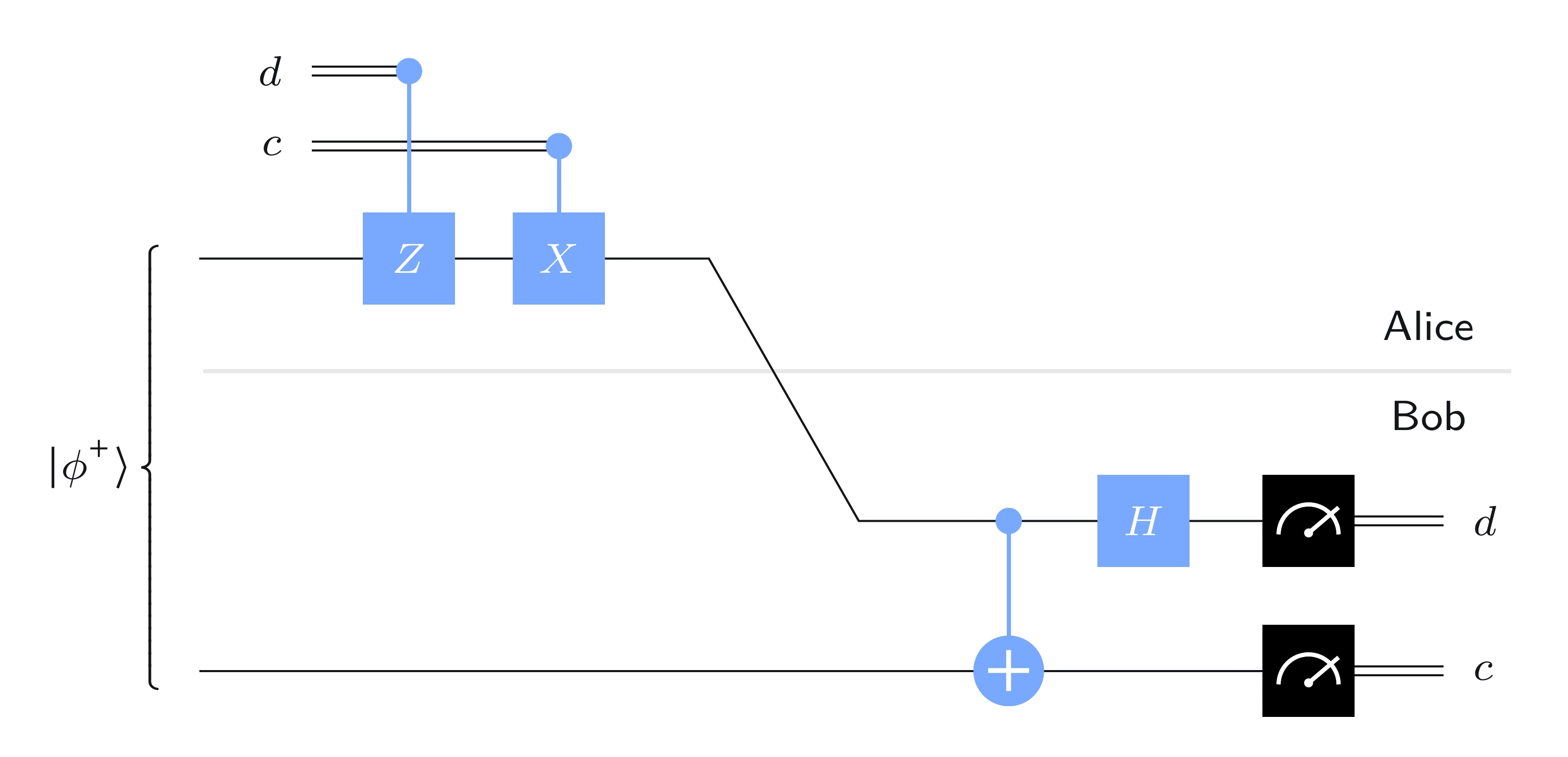
Alice가 수행하는 동작을 말로 설명하면 다음과 같습니다.

$d=1$ 이면 Alice는 자신의 qubit $\mathsf{A}$ 에 $Z$ Gate를 적용합니다 ( $d=0$ 이면 아무것도 하지 않습니다).
$c=1$ 이면 Alice는 자신의 qubit $\mathsf{A}$ 에 $X$ Gate를 적용합니다 ( $c=0$ 이면 아무것도 하지 않습니다).

그런 다음 Alice는 자신의 qubit $\mathsf{A}$ 를 Bob에게 전송합니다.

Bob은 qubit $\mathsf{A}$ 를 받으면, 먼저 $\mathsf{A}$ 를 제어 비트로 하고 $\mathsf{B}$ 를 대상으로 하는 CNOT Gate를 수행한 뒤 $,\mathsf{A}$ 에 Hadamard Gate를 적용합니다. 그런 다음 표준 기저 측정으로 $\mathsf{B}$ 를 측정하여 $c$ 를 얻고 $,\mathsf{A}$ 를 측정하여 $d$ 를 얻습니다.

분석

이 프로토콜의 기본 아이디어는 간단합니다. Alice는 Bob과 공유할 Bell 상태를 선택하고, Bob에게 자신의 Qubit을 전송하면, Bob은 Alice가 어떤 Bell 상태를 선택했는지 측정을 통해 알아냅니다.

즉, 처음에 $\vert\phi^+\rangle$ 를 공유하고, 비트 $c$ 와 $d$ 에 따라 Alice는 자신의 qubit $\mathsf{A}$ 에 $\mathbb{I}$ , $X$ , $Z$ , 또는 $XZ$ 를 적용하여 이 상태를 유지하거나 다른 Bell 상태 중 하나로 변환합니다.

\begin{aligned} (\mathbb{I} \otimes \mathbb{I}) \vert \phi^+ \rangle & = \vert \phi^+\rangle \\ (\mathbb{I} \otimes Z) \vert \phi^+ \rangle & = \vert \phi^-\rangle \\ (\mathbb{I} \otimes X) \vert \phi^+ \rangle & = \vert \psi^+\rangle \\ (\mathbb{I} \otimes XZ) \vert \phi^+ \rangle & = \vert \psi^-\rangle \end{aligned}

Bob의 동작이 네 개의 Bell 상태에 미치는 효과는 다음과 같습니다.

\begin{aligned} \vert \phi^+\rangle & \mapsto \vert 00\rangle\\ \vert \phi^-\rangle & \mapsto \vert 01\rangle\\ \vert \psi^+\rangle & \mapsto \vert 10\rangle\\ \vert \psi^-\rangle & \mapsto -\vert 11\rangle\\ \end{aligned}

이는 Bob의 연산 결과를 각 상태별로 직접 계산하여 확인할 수 있습니다.

따라서 Bob이 측정을 수행하면 Alice가 선택한 Bell 상태를 파악할 수 있습니다. 프로토콜이 올바르게 동작하는지 검증하려면 각 경우를 확인하면 됩니다.

$cd = 00$ 이면, Bob이 $\mathsf{A}$ 를 받았을 때 $(\mathsf{B},\mathsf{A})$ 의 상태는 $\vert \phi^+\rangle$ 입니다. Bob은 이 상태를 $\vert 00\rangle$ 으로 변환하고 $cd = 00$ 을 얻습니다.
$cd = 01$ 이면, Bob이 $\mathsf{A}$ 를 받았을 때 $(\mathsf{B},\mathsf{A})$ 의 상태는 $\vert \phi^-\rangle$ 입니다. Bob은 이 상태를 $\vert 01\rangle$ 으로 변환하고 $cd = 01$ 을 얻습니다.
$cd = 10$ 이면, Bob이 $\mathsf{A}$ 를 받았을 때 $(\mathsf{B},\mathsf{A})$ 의 상태는 $\vert \psi^+\rangle$ 입니다. Bob은 이 상태를 $\vert 10\rangle$ 으로 변환하고 $cd = 10$ 을 얻습니다.
$cd = 11$ 이면, Bob이 $\mathsf{A}$ 를 받았을 때 $(\mathsf{B},\mathsf{A})$ 의 상태는 $\vert \psi^-\rangle$ 입니다. Bob은 이 상태를 $-\vert 11\rangle$ 으로 변환하고 $cd = 11$ 을 얻습니다. (마이너스 1 위상 인수는 여기서 아무런 영향을 미치지 않습니다.)

초밀집 부호화 구현

다음은 전송할 비트에 따라 Circuit을 직접 지정하는 초밀집 부호화의 간단한 구현입니다. 먼저 전송할 두 비트를 선택합니다. (나중에 무작위로 선택하겠지만, 지금은 임의의 값을 사용합니다.)

c = "1"
d = "0"

이제 이에 따라 Circuit을 구성합니다. 여기서는 Qiskit이 Qubit의 기본 이름을 사용하도록 합니다. 상단 Qubit은 $\mathsf{q}_0$ , 하단 Qubit은 $\mathsf{q}_1$ 입니다.

protocol = QuantumCircuit(2)

# Prepare ebit used for superdense coding
protocol.h(0)
protocol.cx(0, 1)
protocol.barrier()

# Alice's operations
if d == "1":
    protocol.z(0)
if c == "1":
    protocol.x(0)
protocol.barrier()

# Bob's actions
protocol.cx(0, 1)
protocol.h(0)
protocol.measure_all()

display(protocol.draw(output="mpl"))

이전 코드 셀의 출력

새로 등장한 기능은 measure_all 함수로, 모든 Qubit을 측정하여 결과를 단일 고전 레지스터에 저장합니다(이 경우 두 비트가 됩니다).

Aer 시뮬레이터를 실행하면 예상된 출력이 나옵니다.

result = AerSimulator().run(protocol).result()
statistics = result.get_counts()

for outcome, frequency in statistics.items():
    print(f"Measured {outcome} with frequency {frequency}")

display(plot_histogram(statistics))

Measured 10 with frequency 1024

이전 코드 셀의 출력

이번에는 추가 Qubit을 무작위 비트 생성기로 사용하여, 공정한 동전을 던지는 것처럼 $c$ 와 $d$ 를 무작위로 선택한 뒤 초밀집 부호화 프로토콜을 실행해 보겠습니다.

rbg = QuantumRegister(1, "coin")
ebit0 = QuantumRegister(1, "A")
ebit1 = QuantumRegister(1, "B")

Alice_c = ClassicalRegister(1, "Alice c")
Alice_d = ClassicalRegister(1, "Alice d")

test = QuantumCircuit(rbg, ebit0, ebit1, Alice_d, Alice_c)

# Initialize the ebit
test.h(ebit0)
test.cx(ebit0, ebit1)
test.barrier()

# Use the 'coin' qubit twice to generate Alice's bits c and d.
test.h(rbg)
test.measure(rbg, Alice_c)
test.h(rbg)
test.measure(rbg, Alice_d)
test.barrier()

# Now the protocol runs, starting with Alice's actions, which depend
# on her bits.
with test.if_test((Alice_d, 1), label="Z"):
    test.z(ebit0)
with test.if_test((Alice_c, 1), label="X"):
    test.x(ebit0)
test.barrier()

# Bob's actions
test.cx(ebit0, ebit1)
test.h(ebit0)
test.barrier()

Bob_c = ClassicalRegister(1, "Bob c")
Bob_d = ClassicalRegister(1, "Bob d")
test.add_register(Bob_d)
test.add_register(Bob_c)
test.measure(ebit0, Bob_d)
test.measure(ebit1, Bob_c)

display(test.draw(output="mpl"))

이전 코드 셀의 출력

Aer 시뮬레이터를 실행하면 결과가 나타납니다. Alice와 Bob의 고전 비트는 항상 일치합니다.

result = AerSimulator().run(test).result()
statistics = result.get_counts()
display(plot_histogram(statistics))

이전 코드 셀의 출력

Qiskit 구현

위에서 정의한 양자 전략과 함께 CHSH 게임을 Qiskit으로 다음과 같이 구현할 수 있습니다.

먼저 게임 자체를 정의합니다. 임의의 전략을 인수로 전달할 수 있도록 구성합니다.

def chsh_game(strategy):
    # This function runs the CHSH game, using the strategy (a function
    # from two bits to two bits), returning 1 for a win and 0 for a loss.

    # Choose x and y randomly
    x, y = random.randint(0, 1), random.randint(0, 1)

    # Use the strategy to determine a and b
    a, b = strategy(x, y)

    # Decide if the strategy wins or loses
    if (a != b) == (x & y):
        return 1  # Win
    return 0  # Lose

이제 Alice와 Bob의 질문에 따라 Circuit을 출력하는 함수를 만들겠습니다. 단순함을 위해 Qubit의 기본 이름을 사용하고, Alice와 Bob의 동작에는 내장된 $R_y(\theta)$ Gate를 사용합니다.

def chsh_circuit(x, y):
    # This function creates a `QuantumCircuit` implementing the quantum
    # strategy described above (including the e-bit preparation).

    qc = QuantumCircuit(2, 2)

    # Prepare an e-bit
    qc.h(0)
    qc.cx(0, 1)
    qc.barrier()

    # Alice's actions
    if x == 0:
        qc.ry(0, 0)
    else:
        qc.ry(-pi / 2, 0)
    qc.measure(0, 0)

    # Bob's actions
    if y == 0:
        qc.ry(-pi / 4, 1)
    else:
        qc.ry(pi / 4, 1)
    qc.measure(1, 1)

    return qc

다음은 질문이 무엇이냐에 따른 네 가지 가능한 Circuit입니다.

# Draw the four possible circuits

print("(x,y) = (0,0)")
display(chsh_circuit(0, 0).draw(output="mpl"))

print("(x,y) = (0,1)")
display(chsh_circuit(0, 1).draw(output="mpl"))

print("(x,y) = (1,0)")
display(chsh_circuit(1, 0).draw(output="mpl"))

print("(x,y) = (1,1)")
display(chsh_circuit(1, 1).draw(output="mpl"))

(x,y) = (0,0)

Output of the previous code cell

(x,y) = (0,1)

Output of the previous code cell

(x,y) = (1,0)

Output of the previous code cell

(x,y) = (1,1)

Output of the previous code cell

이제 Aer 시뮬레이터를 사용하여 주어진 입력 쌍 $(x,y)$ 에 대해 Circuit을 한 번 실행하는 작업을 생성합니다.

def quantum_strategy(x, y):
    # This function runs the appropriate quantum circuit defined above
    # one time and returns the measurement results

    # Setting `shots=1` to run the circuit once
    result = AerSimulator().run(chsh_circuit(x, y), shots=1).result()
    statistics = result.get_counts()

    # Determine the output bits and return them
    bits = list(statistics.keys())[0]
    a, b = bits[0], bits[1]
    return a, b

마지막으로, 게임을 1000번 진행하고 전략이 이기는 비율을 계산합니다.

NUM_GAMES = 1000
TOTAL_SCORE = 0

for _ in range(NUM_GAMES):
    TOTAL_SCORE += chsh_game(quantum_strategy)

print("Fraction of games won:", TOTAL_SCORE / NUM_GAMES)

Fraction of games won: 0.867

고전적 전략도 정의하여 얼마나 잘 작동하는지 확인할 수 있습니다. 이것은 하나의 전략일 뿐이며 — 코드를 변경하면 다른 전략도 테스트할 수 있습니다 — 하지만 이 전략은 최적의 고전적 전략 중 하나입니다.

def classical_strategy(x, y):
    # This function implements just one example of an optimal classical
    # strategy for the CHSH game. Other classical strategies can be
    # implemented by changing the bit values assigned to a and b.

    # Alice's answer
    if x == 0:
        a = 0
    elif x == 1:
        a = 1

    # Bob's answer
    if y == 0:
        b = 1
    elif y == 1:
        b = 0

    return a, b

다시 게임을 1000번 진행하여 얼마나 잘 작동하는지 확인합니다.

NUM_GAMES = 1000
TOTAL_SCORE = 0

for _ in range(NUM_GAMES):
    TOTAL_SCORE += chsh_game(classical_strategy)

print("Fraction of games won:", TOTAL_SCORE / NUM_GAMES)

Fraction of games won: 0.747

무작위성이 관여하지만, 1000번 실행 후 통계가 크게 벗어날 가능성은 매우 낮습니다. 양자 전략은 약 85%의 승률을 보이는 반면, 고전적 전략은 약 75% 이상 이길 수 없습니다.

초밀집 부호화​

프로토콜​

분석​

초밀집 부호화 구현​

Qiskit 구현​

초밀집 부호화

프로토콜

분석

초밀집 부호화 구현

Qiskit 구현