양자 변분 Circuit과 양자 신경망
이 강의에서는 데이터 분류 작업을 위한 여러 변분 양자 회로를 구현합니다. 이를 변분 양자 분류기(VQC)라고 합니다. 한때는 고전 신경망과의 유사성을 들어 VQC의 일부를 양자 신경망(QNN)이라고 부르는 것이 일반적이었습니다. 실제로 컨볼루션 레이어와 같이 고전 신경망에서 차용한 구조가 VQC에서 중요한 역할을 하는 경우가 있습니다. 이처럼 유사성이 강한 경우에는 QNN이 유용한 표현일 수 있습니다. 하지만 매개변수화된 양자 회로가 반드시 신경망의 일반적인 구조를 따를 필요는 없습니다. 예를 들어, 모든 데이터를 첫 번째(입력) 레이어에서 로드할 필요는 없으며, 일부 데이터를 첫 번째 레이어에서 로드하고 몇 가지 Gate를 적용한 후 추가 데이터를 로드하는 방식(데이터 "재업로드"라고 불리는 과정)도 가능합니다. 따라서 QNN은 매개변수화된 양자 회로의 부분 집합으로 생각해야 하며, 고전 신경망과의 유사성에만 얽매여 유용한 양자 회로를 탐색하는 것을 제한해서는 안 됩니다.
이 강의에서 다루는 데이터셋은 수평 및 수직 줄무늬가 포함된 이미지로 구성되며, 목표는 줄의 방향에 따라 새로운 이미지를 두 범주 중 하나로 분류하는 것입니다. 이를 VQC를 사용하여 수행합니다. 진행하면서 계산을 개선하고 확장하는 방법도 살펴봅니다. 여기서 사용하는 데이터셋은 고전적으로 분류하기가 매우 쉽습니다. 단순함 때문에 선택한 것으로, 이 문제의 양자적 측면에 집중하고 데이터셋의 특성이 양자 회로의 어떤 부분으로 변환될 수 있는지 살펴보기 위함입니다. 고전 알고리즘이 매우 효율적인 이처럼 단순한 경우에는 양자 속도 향상을 기대하는 것이 합리적이지 않습니다.
이 강의를 마치면 다음을 할 수 있어야 합니다:
- 이미지에서 양자 Circuit으로 데이터 로드하기
- VQC(또는 QNN)용 Ansatz를 구성하고 문제에 맞게 조정하기
- VQC/QNN을 훈련하고 테스트 데이터에서 정확한 예측에 사용하기
- 문제를 확장하고 현재 양자 컴퓨터의 한계 인식하기
데이터 생성
먼저 데이터를 구성하겠습니다. 데이터셋은 Qiskit 패턴 프레임워크의 일부로 명시적으로 생성되지 않는 경우가 많습니다. 하지만 데이터 유형과 준비는 머신러닝에 양자 컴퓨팅을 성공적으로 적용하는 데 매우 중요합니다. 아래 코드는 정해진 픽셀 크기의 이미지 데이터셋을 정의합니다. 이미지의 전체 행 또는 열 하나는 값이 할당되고, 나머지 픽셀에는 구간 의 무작위 값이 할당됩니다. 무작위 값은 데이터의 노이즈입니다. 코드를 훑어보며 이미지가 어떻게 생성되는지 이해해 보세요. 나중에 이미지를 더 크게 확장할 것입니다.
# Added by doQumentation — required packages for this notebook
!pip install -q matplotlib numpy qiskit qiskit-ibm-runtime scipy scikit-learn
# This code defines the images to be classified:

import numpy as np

# Total number of "pixels"/qubits
size = 8
# One dimension of the image (called vertical, but it doesn't matter). Must be a divisor of `size`
vert_size = 2
# The length of the line to be detected (yellow). Must be less than or equal to the smallest
# dimension of the image (`<=min(vert_size,size/vert_size)`
line_size = 2

def generate_dataset(num_images):
    images = []
    labels = []
    hor_array = np.zeros((size - (line_size - 1) * vert_size, size))
    ver_array = np.zeros((round(size / vert_size) * (vert_size - line_size + 1), size))

    j = 0
    for i in range(0, size - 1):
        if i % (size / vert_size) <= (size / vert_size) - line_size:
            for p in range(0, line_size):
                hor_array[j][i + p] = np.pi / 2
            j += 1

    # Make two adjacent entries pi/2, then move down to the next row. Careful to avoid the "pixels"
    # at size/vert_size - linesize, because we want to fold this list into a grid.

    j = 0
    for i in range(0, round(size / vert_size) * (vert_size - line_size + 1)):
        for p in range(0, line_size):
            ver_array[j][i + p * round(size / vert_size)] = np.pi / 2
        j += 1

    # Make entries pi/2, spaced by the length/rows, so that when folded,
    # the entries appear on top of each other.

    for n in range(num_images):
        rng = np.random.randint(0, 2)
        if rng == 0:
            labels.append(-1)
            random_image = np.random.randint(0, len(hor_array))
            images.append(np.array(hor_array[random_image]))

        elif rng == 1:
            labels.append(1)
            random_image = np.random.randint(0, len(ver_array))
            images.append(np.array(ver_array[random_image]))
            # Randomly select 0 or 1 for a horizontal or vertical array, assign the corresponding
            # label.

        # Create noise
        for i in range(size):
            if images[-1][i] == 0:
                images[-1][i] = np.random.rand() * np.pi / 4
    return images, labels

hor_size = round(size / vert_size)
위 코드는 이미지에 수직선(+1) 또는 수평선(-1)이 포함되어 있는지를 나타내는 레이블도 생성했습니다. 이제 sklearn을 사용하여 100개의 이미지 데이터셋을 훈련 세트와 테스트 세트(해당 레이블 포함)로 분할합니다. 여기서는 데이터셋의 를 훈련에 사용하고 나머지 는 테스트용으로 보류합니다.
from sklearn.model_selection import train_test_split

np.random.seed(42)
images, labels = generate_dataset(200)

train_images, test_images, train_labels, test_labels = train_test_split(
    images, labels, test_size=0.3, random_state=246
)
데이터셋의 몇 가지 요소를 그려서 이 줄들이 어떻게 생겼는지 확인해 보겠습니다:
import matplotlib.pyplot as plt

# Make subplot titles so we can identify categories
titles = []
for i in range(8):
    title = "category: " + str(train_labels[i])
    titles.append(title)

# Generate a figure with nested images using subplots.
fig, ax = plt.subplots(4, 2, figsize=(10, 6), subplot_kw={"xticks": [], "yticks": []})

for i in range(8):
    ax[i // 2, i % 2].imshow(
        train_images[i].reshape(vert_size, hor_size),
        aspect="equal",
    )
    ax[i // 2, i % 2].set_title(titles[i])
plt.subplots_adjust(wspace=0.1, hspace=0.3)

각 이미지는 간단한 리스트 형태로 train_labels에 레이블과 함께 저장되어 있습니다:
print(train_labels[:8])
[1, 1, 1, 1, -1, 1, 1, 1]
변분 양자 분류기: 첫 번째 시도
Qiskit Patterns 1단계: 문제를 양자 Circuit으로 매핑하기
목표는 매개변수 를 가진 함수 를 찾아, 데이터 벡터 / 이미지 를 올바른 범주로 매핑하는 것입니다: . 이는 각각 고유한 목적을 가진 몇 개의 레이어로 식별할 수 있는 소수의 레이어를 가진 VQC를 사용하여 달성됩니다:
여기서 는 인코딩 Circuit으로, 이전 강의에서 살펴보았듯이 여러 가지 옵션이 있습니다. 는 변분(훈련 가능한) Circuit 블록이고, 는 훈련될 매개변수 집합입니다. 이 매개변수들은 고전적인 최적화 알고리즘에 의해 변화하여 양자 Circuit이 이미지를 가장 잘 분류하는 매개변수 집합을 찾습니다. 이 변분 Circuit은 때로 "ansatz"라고도 불립니다. 마지막으로, 는 Estimator 기본 요소를 사용하여 추정될 관측량입니다. 레이어가 반드시 이 순서로 오거나 완전히 분리될 필요는 없습니다. 기술적으로 동기화된 임의의 순서로 여러 개의 변분 및/또는 인코딩 레이어를 가질 수 있습니다.
먼저 데이터를 인코딩할 feature map을 선택합니다. 다른 feature mapping에 비해 Circuit 깊이를 낮게 유지하는 z_feature_map을 사용하겠습니다.
from qiskit.circuit.library import z_feature_map

# One qubit per data feature
num_qubits = len(train_images[0])

# Data encoding
# Note that qiskit orders parameters alphabetically. We assign the parameter prefix "a" to ensure
# our data encoding goes to the first part of the circuit, the feature mapping.
feature_map = z_feature_map(num_qubits, parameter_prefix="a")
이제 훈련할 ansatz를 결정해야 합니다. ansatz를 선택할 때 고려할 사항이 많습니다. 완전한 설명은 이 소개의 범위를 벗어나므로, 여기서는 몇 가지 고려 사항의 범주만 간단히 짚어보겠습니다.
- 하드웨어: 현대의 모든 양자 컴퓨터는 고전적인 컴퓨터보다 오류가 발생하기 쉽고 노이즈에 더 취약합니다. 지나치게 깊은 (특히 트랜스파일된 2-Qubit 깊이에서) ansatz를 사용하면 좋은 결과를 얻을 수 없습니다. 관련된 문제로, 양자 컴퓨터에는 일부 물리적 Qubit들이 서로 인접해 있고 다른 것들은 매우 멀리 떨어져 있는 레이아웃이 있습니다. 인접한 Qubit을 얽히게 하는 것은 깊이를 크게 늘리지 않지만, 매우 멀리 떨어진 Qubit을 얽히게 하면 깊이가 상당히 증가할 수 있습니다. 이는 인접한 Qubit으로 정보를 이동시키기 위해 swap Gate를 삽입해야 하기 때문입니다.
- 문제: ansatz를 안내할 수 있는 문제에 대한 정보가 있다면 활용하세요. 예를 들어, 이 강의의 데이터는 수평선과 수직선 이미지로 구성되어 있습니다. 인접한 색상/값 간의 어떤 상관관계가 수평선 또는 수직선 이미지를 식별하는지 생각해 볼 수 있습니다. ansatz의 어떤 속성이 인접한 픽셀 간의 이러한 상관관계에 해당할까요? 이 강의의 후반부에서 이 점을 더 기술적으로 다시 살펴볼 것입니다. 하지만 지금은, 인접한 픽셀에 해당하는 qubit 간의 얽힘과 CNOT Gate를 포함하는 것이 좋은 아이디어로 보인다고만 말씀드리겠습니다. 더 큰 그림에서, 문제가 실제로 양자 Circuit을 사용하여 가장 잘 해결되는지, 또는 동일한 성능을 낼 수 있는 고전적인 알고리즘이 있는지 고려하세요.
- 매개변수의 수: Circuit에서 독립적으로 매개변수화된 각 양자 Gate는 고전적으로 최적화해야 할 공간을 늘리며, 이는 수렴을 느리게 합니다. 하지만 문제가 확장됨에 따라 barren plateaus에 직면할 수 있습니다. 이 용어는 변분 양자 알고리즘의 최적화 지형이 문제 크기가 증가함에 따라 지수적으로 평평하고 특징 없어지는 현상을 의미합니다. 이로 인해 기울기가 사라져 알고리즘을 효과적으로 훈련하기 어려워집니다[1]. Barren plateaus는 VQC/QNN과 같은 변분 양자 알고리즘과 관련이 있습니다. 증가하는 매개변수 수만이 barren plateaus를 피하는 데 고려해야 할 유일한 요소가 아니라는 점에 주목해야 합니다. 전역 비용 함수와 무작위 매개변수 초기화도 고려 사항에 포함됩니다.
이 강의에서는 ansatz 구성의 좋은 사례를 몇 가지 간단히 살펴볼 것입니다. 먼저 아래의 ansatz를 시도해 보겠습니다. 나중에 다시 수정할 것입니다.
# Import the necessary packages
from qiskit import QuantumCircuit
from qiskit.circuit import ParameterVector

# Initialize the circuit using the same number of qubits as the image has pixels
qnn_circuit = QuantumCircuit(size)

# We choose to have two variational parameters for each qubit.
params = ParameterVector("θ", length=2 * size)

# A first variational layer:
for i in range(size):
    qnn_circuit.ry(params[i], i)

# Here is a list of qubit pairs between which we want CNOT gates.
# The choice of these is not yet obvious.
qnn_cnot_list = [[0, 1], [1, 2], [2, 3]]

for i in range(len(qnn_cnot_list)):
    qnn_circuit.cx(qnn_cnot_list[i][0], qnn_cnot_list[i][1])

# The second variational layer:
for i in range(size):
    qnn_circuit.rx(params[size + i], i)

# Check the circuit depth, and the two-qubit gate depth
print(qnn_circuit.decompose().depth())
print(
    f"2+ qubit depth: {qnn_circuit.decompose().depth(lambda instr: len(instr.qubits) > 1)}"
)

# Draw the circuit
qnn_circuit.draw("mpl")
5
2+ qubit depth: 3
┌──────────┐             ┌──────────┐
q_0: ┤ Ry(θ[0]) ├──────■──────┤ Rx(θ[8]) ├─────────────────────────
     ├──────────┤    ┌─┴─┐    └──────────┘┌──────────┐
q_1: ┤ Ry(θ[1]) ├────┤ X ├─────────■──────┤ Rx(θ[9]) ├─────────────
     ├──────────┤    └───┘       ┌─┴─┐    └──────────┘┌───────────┐
q_2: ┤ Ry(θ[2]) ├────────────────┤ X ├─────────■──────┤ Rx(θ[10]) ├
     ├──────────┤                └───┘       ┌─┴─┐    ├───────────┤
q_3: ┤ Ry(θ[3]) ├────────────────────────────┤ X ├────┤ Rx(θ[11]) ├
     ├──────────┤┌───────────┐               └───┘    └───────────┘
q_4: ┤ Ry(θ[4]) ├┤ Rx(θ[12]) ├─────────────────────────────────────
     ├──────────┤├───────────┤
q_5: ┤ Ry(θ[5]) ├┤ Rx(θ[13]) ├─────────────────────────────────────
     ├──────────┤├───────────┤
q_6: ┤ Ry(θ[6]) ├┤ Rx(θ[14]) ├─────────────────────────────────────
     ├──────────┤├───────────┤
q_7: ┤ Ry(θ[7]) ├┤ Rx(θ[15]) ├─────────────────────────────────────
     └──────────┘└───────────┘
데이터 인코딩과 변분 Circuit이 준비되었으니, 이를 결합하여 완전한 ansatz를 구성할 수 있습니다. 이 경우, 양자 Circuit의 구성 요소는 신경망의 구성 요소와 꽤 유사합니다. 는 이미지에서 입력값을 로드하는 레이어와 가장 유사하고, 는 가변 "가중치"의 레이어와 같습니다. 이 비유가 이 경우에 성립하므로, 일부 명명 규칙에 "qnn"을 사용하고 있습니다. 하지만 이 비유가 VQC 탐색을 제한해서는 안 됩니다.

# QNN ansatz
ansatz = qnn_circuit

# Combine the feature map with the ansatz
full_circuit = QuantumCircuit(num_qubits)
full_circuit.compose(feature_map, range(num_qubits), inplace=True)
full_circuit.compose(ansatz, range(num_qubits), inplace=True)

# Display the circuit
full_circuit.decompose().draw("mpl", style="clifford", fold=-1)

이제 관측량을 정의해야 합니다. 비용 함수에서 사용할 것입니다. Estimator를 사용하여 이 관측량의 기댓값을 구할 것입니다. 문제에 잘 맞는 ansatz를 선택했다면, 각 Qubit은 분류에 관련된 정보를 포함하게 됩니다. Circuit의 일부 Qubit에서만 측정이 필요하도록 정보를 더 적은 Qubit으로 결합하는 레이어(합성곱 신경망에서처럼 합성곱 레이어라고 불림)를 추가할 수 있습니다. 또는 각 Qubit에서 일부 속성을 측정할 수도 있습니다. 여기서는 후자를 선택하여 각 Qubit에 Z 연산자를 포함합니다. 를 선택하는 것이 특별한 이유는 없지만, 다음과 같은 이유로 잘 동기화되어 있습니다:
- 이진 분류 작업이며, 측정은 두 가지 가능한 결과를 산출할 수 있습니다.
- 의 고유값 ()은 적절히 잘 분리되어 있으며, Estimator 결과를 [-1, +1] 구간에 있게 하여 0을 단순한 컷오프 값으로 사용할 수 있습니다.
- 추가적인 Gate 오버헤드 없이 Pauli Z 기저에서 측정하는 것이 간단합니다.
따라서 Z는 매우 자연스러운 선택입니다.
from qiskit.quantum_info import SparsePauliOp

observable = SparsePauliOp.from_list([("Z" * (num_qubits), 1)])
양자 Circuit과 추정하려는 관측량이 준비되었습니다. 이제 이 Circuit을 실행하고 최적화하기 위한 몇 가지가 필요합니다. 먼저, 순방향 패스를 실행하는 함수가 필요합니다. 아래 함수는 input_params와 weight_params를 별도로 받는다는 점에 주목하세요. 전자는 이미지의 데이터를 설명하는 정적 매개변수 집합이고, 후자는 최적화될 가변 매개변수 집합입니다.
from qiskit.primitives import BaseEstimatorV2
from qiskit.quantum_info.operators.base_operator import BaseOperator

def forward(
    circuit: QuantumCircuit,
    input_params: np.ndarray,
    weight_params: np.ndarray,
    estimator: BaseEstimatorV2,
    observable: BaseOperator,
) -> np.ndarray:
    """
    Forward pass of the neural network.

    Args:
        circuit: circuit consisting of data loader gates and the neural network ansatz.
        input_params: data encoding parameters.
        weight_params: neural network ansatz parameters.
        estimator: EstimatorV2 primitive.
        observable: a single observable to compute the expectation over.

    Returns:
        expectation_values: an array (for one observable) or a matrix (for a sequence of observables) of expectation values.
        Rows correspond to observables and columns to data samples.
    """
    num_samples = input_params.shape[0]
    weights = np.broadcast_to(weight_params, (num_samples, len(weight_params)))
    params = np.concatenate((input_params, weights), axis=1)
    pub = (circuit, observable, params)
    job = estimator.run([pub])
    result = job.result()[0]
    expectation_values = result.data.evs

    return expectation_values
손실 함수
다음으로, 예측된 레이블과 계산된 레이블 간의 차이를 계산하는 손실 함수가 필요합니다. 이 함수는 알고리즘이 예측한 레이블과 정확한 레이블을 받아 평균 제곱 차이를 반환합니다. 손실 함수에는 여러 종류가 있습니다. 여기서는 MSE를 예시로 선택했습니다.
def mse_loss(predict: np.ndarray, target: np.ndarray) -> np.ndarray:
    """
    Mean squared error (MSE).

    prediction: predictions from the forward pass of neural network.
    target: true labels.

    output: MSE loss.
    """
    if len(predict.shape) <= 1:
        return ((predict - target) ** 2).mean()
    else:
        raise AssertionError("input should be 1d-array")
고전적 최적화기에서 사용하기 위해 가변 매개변수(가중치)의 함수인 약간 다른 손실 함수도 정의해 봅시다. 이 함수는 ansatz 매개변수만을 입력으로 받습니다. 순방향 패스와 손실에 필요한 다른 변수들은 전역 매개변수로 설정됩니다. 최적화기는 다른 가중치를 샘플링하고 비용/손실 함수의 출력을 낮추려 시도함으로써 모델을 훈련시킵니다.
def mse_loss_weights(weight_params: np.ndarray) -> np.ndarray:
    """
    Cost function for the optimizer to update the ansatz parameters.

    weight_params: ansatz parameters to be updated by the optimizer.

    output: MSE loss.
    """
    predictions = forward(
        circuit=circuit,
        input_params=input_params,
        weight_params=weight_params,
        estimator=estimator,
        observable=observable,
    )

    cost = mse_loss(predict=predictions, target=target)
    objective_func_vals.append(cost)

    global iter
    if iter % 50 == 0:
        print(f"Iter: {iter}, loss: {cost}")
    iter += 1

    return cost
위에서 고전적인 최적화기 사용에 대해 언급했습니다. 비용 함수를 최소화하기 위해 가중치를 탐색할 때 COBYLA 최적화기를 사용할 것입니다:
from scipy.optimize import minimize
비용 함수를 위한 초기 전역 변수를 설정합니다.
# Globals
circuit = full_circuit
observables = observable
# input_params = train_images_batch
# target = train_labels_batch
objective_func_vals = []
iter = 0
Qiskit Patterns 2단계: 양자 실행을 위한 문제 최적화
실행할 Backend를 선택하는 것으로 시작합니다. 여기서는 가장 한가한 Backend를 사용하겠습니다.
from qiskit_ibm_runtime import QiskitRuntimeService

service = QiskitRuntimeService()
backend = service.least_busy(operational=True, simulator=False)
print(backend.name)
ibm_brisbane
여기서는 optimization_level을 지정하고 dynamical decoupling을 추가하여 실제 Backend에서 실행할 수 있도록 Circuit을 최적화합니다. 아래 코드는 qiskit.transpiler의 프리셋 패스 매니저를 사용하여 패스 매니저를 생성합니다.
from qiskit.circuit.library import XGate
from qiskit.transpiler import PassManager
from qiskit.transpiler.passes import (
    ALAPScheduleAnalysis,
    ConstrainedReschedule,
    PadDynamicalDecoupling,
)
from qiskit.transpiler.preset_passmanagers import generate_preset_pass_manager

target = backend.target

pm = generate_preset_pass_manager(target=target, optimization_level=3)
pm.scheduling = PassManager(
    [
        ALAPScheduleAnalysis(target=target),
        ConstrainedReschedule(
            acquire_alignment=target.acquire_alignment,
            pulse_alignment=target.pulse_alignment,
            target=target,
        ),
        PadDynamicalDecoupling(
            target=target,
            dd_sequence=[XGate(), XGate()],
            pulse_alignment=target.pulse_alignment,
        ),
    ]
)
이제 패스 매니저를 Circuit에 적용합니다. 이로 인해 발생하는 레이아웃 변경 사항은 observable에도 적용해야 합니다. 매우 큰 Circuit의 경우, Circuit 최적화에 사용되는 휴리스틱이 항상 가장 좋고 얕은 Circuit을 만들어 내지는 않을 수 있습니다. 그런 경우에는 이러한 패스 매니저를 여러 번 실행하여 최선의 Circuit을 사용하는 것이 합리적입니다. 이는 나중에 계산을 확장할 때 살펴보겠습니다.
circuit_ibm = pm.run(full_circuit)
observable_ibm = observable.apply_layout(circuit_ibm.layout)
Qiskit Patterns 3단계: Qiskit Primitives를 사용하여 실행
데이터셋을 배치와 에폭 단위로 반복
먼저 시뮬레이터를 사용하여 간단한 디버깅과 오차 추정을 위해 전체 알고리즘을 구현합니다. 이제 원하는 수의 에폭 동안 배치 단위로 전체 데이터셋을 처리하여 양자 신경망을 훈련할 수 있습니다.
from qiskit.primitives import StatevectorEstimator as Estimator

batch_size = 140
num_epochs = 1
num_samples = len(train_images)

# Globals
circuit = full_circuit
estimator = Estimator()  # simulator for debugging
observables = observable
objective_func_vals = []
iter = 0

# Random initial weights for the ansatz
np.random.seed(42)
weight_params = np.random.rand(len(ansatz.parameters)) * 2 * np.pi

for epoch in range(num_epochs):
    for i in range((num_samples - 1) // batch_size + 1):
        print(f"Epoch: {epoch}, batch: {i}")
        start_i = i * batch_size
        end_i = start_i + batch_size
        train_images_batch = np.array(train_images[start_i:end_i])
        train_labels_batch = np.array(train_labels[start_i:end_i])
        input_params = train_images_batch
        target = train_labels_batch
        iter = 0
        res = minimize(
            mse_loss_weights, weight_params, method="COBYLA", options={"maxiter": 100}
        )
        weight_params = res["x"]
Epoch: 0, batch: 0
Iter: 0, loss: 1.0002309063537163
Iter: 50, loss: 0.9434121445008878
Qiskit Patterns 4단계: 후처리 및 고전적 형식으로 결과 반환
테스트 및 정확도
이제 훈련 결과를 해석합니다. 먼저 훈련 세트에 대한 훈련 정확도를 테스트합니다.
import copy
from sklearn.metrics import accuracy_score
from qiskit.primitives import StatevectorEstimator as Estimator  # simulator
# from qiskit_ibm_runtime import EstimatorV2 as Estimator  # real quantum computer

estimator = Estimator()
# estimator = Estimator(backend=backend)

pred_train = forward(circuit, np.array(train_images), res["x"], estimator, observable)
# pred_train = forward(circuit_ibm, np.array(train_images), res['x'], estimator, observable_ibm)

print(pred_train)

pred_train_labels = copy.deepcopy(pred_train)
pred_train_labels[pred_train_labels >= 0] = 1
pred_train_labels[pred_train_labels < 0] = -1
print(pred_train_labels)
print(train_labels)

accuracy = accuracy_score(train_labels, pred_train_labels)
print(f"Train accuracy: {accuracy * 100}%")
[-2.27688499e-02 -1.46227204e-02 -1.73927452e-02  9.93331786e-02
 -4.85553548e-01  1.43558565e-01  8.34567054e-02 -1.40133992e-02
  1.52169596e-01 -1.95082515e-01  8.24373578e-03 -9.90696638e-02
 -3.54268344e-02 -4.77017954e-01  1.38713848e-02 -2.99706215e-01
 -5.78378029e-02  3.25528779e-02 -4.11354239e-02 -1.06483708e-01
  1.53095800e-01  2.90110884e-02  1.25745450e-02  6.46323079e-02
 -1.53538943e-01 -1.57694952e-02 -1.67800067e-02 -1.99820822e-01
  1.70360075e-01  7.86148038e-03 -2.33373818e-02  6.64233020e-02
 -1.14895445e-01 -1.11296215e-01  1.15120303e-01 -2.94096140e-01
 -1.00531392e-03 -1.69209726e-01 -1.26120885e-01  3.26298176e-02
 -1.33517383e-02 -5.86983444e-02 -4.32341361e-01 -4.36509551e-01
 -4.17940102e-02  1.76935235e-03  8.14479984e-03  1.86985655e-01
 -2.75525019e-01 -1.63229907e-03 -1.08571055e-01 -7.37452387e-04
 -6.44440657e-02  6.72812834e-04  2.16785530e-03  1.41381850e-01
 -9.82570410e-02  4.35973325e-01 -7.62261965e-02 -1.86193980e-01
 -1.56971183e-02 -4.02757541e-01 -1.53869367e-01  2.29262129e-02
 -7.02788246e-03  3.65719683e-02  4.68232163e-01  2.36434668e-02
 -2.59520939e-02  3.70550137e-01 -1.19630110e-01 -5.79555318e-02
  2.09554455e-01  5.04689780e-02  7.39494314e-02 -1.77647326e-02
 -1.45407207e-01 -9.54908878e-02  7.56029640e-02 -2.74049696e-02
  3.34885873e-01  1.58546171e-03  1.09339091e-01 -8.84693274e-02
 -2.36450457e-02  1.41892239e-01 -2.34453218e-01 -7.50717757e-02
 -1.13281310e-01 -1.66649414e-01 -3.17224197e-01 -6.38220597e-02
  3.28916563e-02  3.04739203e-02  2.67720196e-02 -1.16485785e-01
 -3.08115732e-02 -2.95372010e-02 -7.54669023e-02  6.20013872e-02
 -3.85258710e-01 -1.16456443e-01 -7.38548075e-02 -3.20558243e-02
 -4.22284741e-02  1.01285659e-01 -1.76949246e-01 -2.02767491e-01
 -1.12407344e-01 -3.81408267e-02 -4.33345231e-01 -9.24507501e-02
 -4.21765393e-02 -6.06533771e-02 -2.22257783e-01 -1.17312535e-01
 -6.74132262e-02 -2.76206274e-01 -9.13971800e-02 -2.27653991e-01
  1.66358563e-01  2.17230774e-04  5.76426304e-02 -2.82079169e-02
 -1.15482051e-01 -3.46716009e-01 -3.21448755e-01 -5.20041405e-02
 -2.16833625e-01 -1.06154654e-02 -7.74854811e-02 -3.28257935e-01
 -7.83242410e-02  1.65547682e-01 -2.55294862e-01 -8.89085025e-02
  4.47581491e-01  1.92351832e-02  2.74083885e-02 -3.61304571e-01]
[-1. -1. -1.  1. -1.  1.  1. -1.  1. -1.  1. -1. -1. -1.  1. -1. -1.  1.
 -1. -1.  1.  1.  1.  1. -1. -1. -1. -1.  1.  1. -1.  1. -1. -1.  1. -1.
 -1. -1. -1.  1. -1. -1. -1. -1. -1.  1.  1.  1. -1. -1. -1. -1. -1.  1.
  1.  1. -1.  1. -1. -1. -1. -1. -1.  1. -1.  1.  1.  1. -1.  1. -1. -1.
  1.  1.  1. -1. -1. -1.  1. -1.  1.  1.  1. -1. -1.  1. -1. -1. -1. -1.
 -1. -1.  1.  1.  1. -1. -1. -1. -1.  1. -1. -1. -1. -1. -1.  1. -1. -1.
 -1. -1. -1. -1. -1. -1. -1. -1. -1. -1. -1. -1.  1.  1.  1. -1. -1. -1.
 -1. -1. -1. -1. -1. -1. -1.  1. -1. -1.  1.  1.  1. -1.]
[1, 1, 1, 1, -1, 1, 1, 1, -1, 1, 1, 1, -1, -1, -1, -1, -1, -1, -1, -1, 1, -1, 1, 1, -1, 1, 1, 1, 1, -1, 1, 1, -1, 1, 1, -1, 1, 1, -1, -1, -1, 1, -1, -1, 1, -1, 1, 1, -1, 1, -1, 1, 1, -1, 1, 1, 1, 1, -1, -1, -1, -1, 1, -1, 1, 1, 1, -1, -1, 1, 1, -1, 1, 1, -1, -1, 1, -1, 1, 1, 1, 1, 1, -1, -1, 1, -1, -1, -1, -1, -1, 1, 1, -1, -1, 1, -1, -1, 1, 1, -1, 1, -1, 1, 1, 1, 1, 1, -1, -1, -1, 1, -1, -1, -1, 1, -1, -1, 1, -1, 1, -1, 1, 1, -1, -1, -1, 1, 1, 1, -1, -1, -1, 1, -1, 1, 1, -1, -1, -1]
Train accuracy: 60.0%
훈련 정확도가 에 불과한데, 이는 분명히 좋지 않은 결과입니다. 테스트 세트에서의 모델 성능이 더 나을 것이라고 기대하기는 어렵습니다. 직접 확인해 보겠습니다.
pred_test = forward(circuit, np.array(test_images), res["x"], estimator, observable)
# pred_test = forward(circuit_ibm, np.array(test_images), res['x'], estimator, observable_ibm)

print(pred_test)

pred_test_labels = copy.deepcopy(pred_test)
pred_test_labels[pred_test_labels >= 0] = 1
pred_test_labels[pred_test_labels < 0] = -1
print(pred_test_labels)
print(test_labels)

accuracy = accuracy_score(test_labels, pred_test_labels)
print(f"Test accuracy: {accuracy * 100}%")
[-2.77978120e-01 -2.62194862e-01  4.59636095e-02 -8.09344165e-02
 -2.97362966e-01  9.22947242e-02  2.06693174e-01  3.31629460e-02
  1.10971762e-03 -2.14602152e-01 -1.62671993e-01 -6.07179155e-04
 -1.59948633e-01 -8.55722523e-02 -1.13057027e-01 -3.00187433e-01
 -2.92832827e-01  7.38580629e-02 -6.03706270e-02 -8.57643552e-02
 -1.52402062e-02 -3.57505447e-01 -3.54890597e-02  1.36534749e-01
 -1.54688180e-01 -2.93714726e-01  1.89548513e-02 -6.15715564e-02
  1.11042670e-01 -2.22861100e-02 -3.84230105e-02  1.67351034e-01
 -8.38766333e-02  2.56348613e-01 -1.10653111e-01 -1.18989476e-01
 -6.75723266e-05 -6.88580547e-02  1.02431393e-02 -2.42125353e-01
 -1.09142367e-01 -1.22540757e-01 -1.63735850e-01  3.93334838e-01
  2.36705685e-01 -2.34259814e-02 -3.91877756e-02 -1.95106746e-01
  1.86707523e-01  4.74775215e-02 -4.24907432e-02 -2.06453265e-01
  4.09184710e-02 -3.54762080e-02 -9.47513112e-02  2.97270112e-01
 -2.99708696e-02  9.93941064e-03 -1.26760302e-01 -1.36183355e-01]
[-1. -1.  1. -1. -1.  1.  1.  1.  1. -1. -1. -1. -1. -1. -1. -1. -1.  1.
 -1. -1. -1. -1. -1.  1. -1. -1.  1. -1.  1. -1. -1.  1. -1.  1. -1. -1.
 -1. -1.  1. -1. -1. -1. -1.  1.  1. -1. -1. -1.  1.  1. -1. -1.  1. -1.
 -1.  1. -1.  1. -1. -1.]
[-1, -1, 1, 1, -1, -1, 1, -1, 1, -1, 1, 1, 1, 1, -1, 1, -1, 1, 1, 1, 1, -1, -1, 1, 1, -1, 1, 1, 1, -1, 1, -1, -1, 1, 1, 1, -1, 1, 1, -1, -1, -1, 1, 1, 1, -1, 1, 1, 1, 1, -1, -1, 1, 1, 1, 1, 1, 1, -1, -1]
Test accuracy: 60.0%
이 모델은 데이터를 제대로 분류하지 못하고 있습니다. 그 이유를 파악해야 하며, 특히 다음 사항들을 확인해야 합니다.
- 훈련을 너무 일찍 중단했나요? 더 많은 최적화 단계가 필요했을까요?
- 잘못된 ansatz를 구성했나요? 이는 다양한 의미를 가질 수 있습니다. 실제 양자 컴퓨터에서 작업할 때, Circuit 깊이는 중요한 고려 사항이 됩니다. 파라미터의 수도 잠재적으로 중요하며, qubit 간의 얽힘도 마찬가지입니다.
- 위 두 가지를 합쳐서, 훈련이 불가능할 정도로 너무 많은 파라미터를 가진 ansatz를 구성했나요?
최적화의 수렴 여부를 확인하는 것부터 시작할 수 있습니다.
obj_func_vals_first = objective_func_vals
# import matplotlib.pyplot as plt

plt.figure(figsize=(12, 6))
plt.plot(obj_func_vals_first, label="first ansatz")
plt.xlabel("iteration")
plt.ylabel("loss")
plt.legend()
plt.show()

최적화 단계를 늘려 옵티마이저가 파라미터 공간의 로컬 최솟값에 갇혀 있는 것은 아닌지 확인해 볼 수도 있습니다. 하지만 충분히 수렴한 것으로 보입니다. 올바르게 분류되지 않은 이미지들을 더 자세히 살펴보고, 어떤 일이 발생하고 있는지 이해해 보겠습니다.
missed = []
for i in range(len(test_labels)):
    if pred_test_labels[i] != test_labels[i]:
        missed.append(test_images[i])
print(len(missed))
24
fig, ax = plt.subplots(12, 2, figsize=(6, 6), subplot_kw={"xticks": [], "yticks": []})
for i in range(len(missed)):
    ax[i // 2, i % 2].imshow(
        missed[i].reshape(vert_size, hor_size),
        aspect="equal",
    )
plt.subplots_adjust(wspace=0.02, hspace=0.025)

여기서 잘못 분류된 이미지의 대다수가 수직선을 포함하고 있음을 알 수 있습니다. 모델이 해당 정보를 제대로 포착하지 못하고 있습니다. 첫 번째 variational Circuit을 기반으로 이미 예상하셨을 수도 있습니다. 더 자세히 살펴보겠습니다.
모델 개선하기
1단계 재검토
문제를 양자 Circuit에 매핑할 때, 인접한 픽셀의 정보가 클래스를 어떻게 결정하는지 명시적으로 고려했어야 했습니다. 수평선을 식별하려면 모든 행에 걸쳐 "픽셀 가 노란색이면 픽셀 도 노란색인가"를 알아야 합니다. 수직선에 대해서도 마찬가지입니다. 하지만 분류가 이진(binary)이므로, 수평선이 감지되지 않으면 수직선으로 간주한다고 단순하게 말할 수도 있습니다. 이전 변분 Circuit에는 qubit(픽셀) 0과 1, 1과 2, 2와 3 사이의 CNOT Gate가 포함되어 있었습니다. 이는 이미지 상단 행의 수평선을 커버하지만, 수직선을 직접 감지하지 못하고, 하단 행을 무시하기 때문에 수평선도 완전히 감지하지 못합니다. 모든 수평선을 완전히 감지하려면 qubit(픽셀) 4와 5, 5와 6, 6과 7 사이에도 유사한 CNOT Gate 세트가 필요합니다. 수직선에 해당하는 qubit 간(예: 0과 4, 또는 2와 6) CNOT Gate를 추가하는 것도 유용할 수 있다는 점을 염두에 두세요. 하지만 먼저 수평선의 존재 여부만 감지하는 것으로 충분한지 확인해 보겠습니다.
# Initialize the circuit using the same number of qubits as the image has pixels
qnn_circuit = QuantumCircuit(size)

# We choose to have two variational parameters for each qubit.
params = ParameterVector("θ", length=2 * size)

# A first variational layer:
for i in range(size):
    qnn_circuit.ry(params[i], i)

# Here is an extended list of qubit pairs between which we want CNOT gates. This now covers all
# pixels connected by horizontal lines.
qnn_cnot_list = [[0, 1], [1, 2], [2, 3], [4, 5], [5, 6], [6, 7]]

for i in range(len(qnn_cnot_list)):
    qnn_circuit.cx(qnn_cnot_list[i][0], qnn_cnot_list[i][1])

# The second variational layer:
for i in range(size):
    qnn_circuit.rx(params[size + i], i)

# Check the circuit depth, and the two-qubit gate depth
print(qnn_circuit.decompose().depth())
print(
    f"2+ qubit depth: {qnn_circuit.decompose().depth(lambda instr: len(instr.qubits) > 1)}"
)

# Combine the feature map and variational circuit
ansatz = qnn_circuit

# Combine the feature map with the ansatz
full_circuit = QuantumCircuit(num_qubits)
full_circuit.compose(feature_map, range(num_qubits), inplace=True)
full_circuit.compose(ansatz, range(num_qubits), inplace=True)

# Display the circuit
full_circuit.decompose().draw("mpl", style="clifford", fold=-1)
5
2+ qubit depth: 3

Circuit의 깊이는 늘어나지 않았습니다. 이미지를 모델링하는 능력이 향상되었는지 확인해 봅시다.
2단계 재검토
실제 양자 Backend에서 실행하려면 이 새로운 Circuit을 Transpiler로 처리해야 합니다. 시뮬레이터에서 변분 Circuit의 수정이 원하는 효과를 가져왔는지 먼저 확인하기 위해 이 단계는 잠시 건너뛰겠습니다. 다음 소절에서 트랜스파일에 대해 더 깊이 살펴볼 것입니다.
3단계 재검토
이제 업데이트된 모델을 훈련 데이터에 적용합니다.
from qiskit.primitives import StatevectorEstimator as Estimator

batch_size = 140
num_epochs = 1
num_samples = len(train_images)

# Globals
circuit = full_circuit
estimator = Estimator()  # simulator for debugging
observables = observable
objective_func_vals = []
iter = 0

# Random initial weights for the ansatz
np.random.seed(42)
weight_params = np.random.rand(len(ansatz.parameters)) * 2 * np.pi

for epoch in range(num_epochs):
    for i in range((num_samples - 1) // batch_size + 1):
        print(f"Epoch: {epoch}, batch: {i}")
        start_i = i * batch_size
        end_i = start_i + batch_size
        train_images_batch = np.array(train_images[start_i:end_i])
        train_labels_batch = np.array(train_labels[start_i:end_i])
        input_params = train_images_batch
        target = train_labels_batch
        iter = 0
        res = minimize(
            mse_loss_weights, weight_params, method="COBYLA", options={"maxiter": 100}
        )
        weight_params = res["x"]
Epoch: 0, batch: 0
Iter: 0, loss: 1.0049762969140237
Iter: 50, loss: 0.8274276543780351
4단계 재검토
먼저 최적화기가 완전히 수렴했는지 확인해 봅시다.
obj_func_vals_revised = objective_func_vals
# import matplotlib.pyplot as plt

plt.figure(figsize=(12, 6))
plt.plot(obj_func_vals_revised, label="revised ansatz")
plt.xlabel("iteration")
plt.ylabel("loss")
plt.legend()
plt.show()

손실 함수가 충분히 많은 스텝 동안 대략적으로 일정한 수준을 유지하지 않았으므로, 완전히 수렴하지 않은 것으로 보입니다. 하지만 손실 함수는 이전 변분 Circuit을 사용했을 때보다 이미 약 60% 낮아졌습니다. 이것이 연구 프로젝트라면 완전한 수렴을 보장해야 하겠지만, 탐색 목적으로는 충분합니다. 훈련 데이터와 테스트 데이터의 정확도를 확인해 봅시다.
from sklearn.metrics import accuracy_score
from qiskit.primitives import StatevectorEstimator as Estimator  # simulator
# from qiskit_ibm_runtime import EstimatorV2 as Estimator  # real quantum computer

estimator = Estimator()
# estimator = Estimator(backend=backend)

pred_train = forward(circuit, np.array(train_images), res["x"], estimator, observable)
# pred_train = forward(circuit_ibm, np.array(train_images), res['x'], estimator, observable_ibm)

print(pred_train)

pred_train_labels = copy.deepcopy(pred_train)
pred_train_labels[pred_train_labels >= 0] = 1
pred_train_labels[pred_train_labels < 0] = -1
print(pred_train_labels)
print(train_labels)

accuracy = accuracy_score(train_labels, pred_train_labels)
print(f"Train accuracy: {accuracy * 100}%")
[ 0.46144755  0.42579688  0.35255977  0.55207273 -0.48578418  0.50805845
  0.44892649  0.6173847  -0.62428139  0.40405121  0.46862421  0.29503395
 -0.5740469  -0.71794562 -0.45022095 -0.45330418 -0.19795258 -0.46821777
 -0.5622049  -0.32114059  0.54947838 -0.4889812   0.28327445  0.58149728
 -0.27026749  0.41328304  0.21119412  0.60108606  0.39204178 -0.24974605
  0.38496469  0.39867586 -0.38946996  0.62616766  0.61212525 -0.49719567
  0.30860002  0.68443904 -0.27505907 -0.41508947 -0.49666422  0.67716994
 -0.54696613 -0.70058779  0.42711815 -0.5285338   0.37678572  0.43888249
 -0.30844464  0.42347715 -0.4250844   0.67324132  0.59914067 -0.45184567
  0.13604098  0.65336342  0.26099853  0.60316559 -0.38743183 -0.54784284
 -0.29549031 -0.45592302  0.41613453 -0.38781528  0.56903087  0.54955451
  0.55532336 -0.3931852  -0.57599675  0.61246236  0.42014135 -0.38171749
  0.56760389  0.45383135 -0.50473943 -0.47551181  0.54221517 -0.64987023
  0.28845851  0.54403865  0.53841148  0.64477078  0.71912049 -0.63178323
 -0.50764757  0.50304637 -0.38099972 -0.27707127 -0.24353841 -0.52045267
 -0.61500665  0.65443173  0.31902266 -0.64969037 -0.4814051   0.47980608
 -0.649786   -0.43048551  0.34562588  0.308998   -0.32454238  0.29558168
 -0.45410187  0.54600712  0.33204827  0.22627804  0.4283921   0.56191874
 -0.25400294 -0.6493613  -0.47445293  0.42272138 -0.35472546 -0.52240474
 -0.45207595  0.40292125 -0.3361856  -0.46620886  0.60202719 -0.56505744
  0.47169796 -0.43577622  0.40689437  0.48869108 -0.39701189 -0.57698634
 -0.39236332  0.31294648  0.41797597  0.63004836 -0.52884541 -0.43805812
 -0.3193499   0.36860211 -0.49190995  0.65000193  0.50260077 -0.56737168
 -0.29693083 -0.40956432]
[ 1.  1.  1.  1. -1.  1.  1.  1. -1.  1.  1.  1. -1. -1. -1. -1. -1. -1.
 -1. -1.  1. -1.  1.  1. -1.  1.  1.  1.  1. -1.  1.  1. -1.  1.  1. -1.
  1.  1. -1. -1. -1.  1. -1. -1.  1. -1.  1.  1. -1.  1. -1.  1.  1. -1.
  1.  1.  1.  1. -1. -1. -1. -1.  1. -1.  1.  1.  1. -1. -1.  1.  1. -1.
  1.  1. -1. -1.  1. -1.  1.  1.  1.  1.  1. -1. -1.  1. -1. -1. -1. -1.
 -1.  1.  1. -1. -1.  1. -1. -1.  1.  1. -1.  1. -1.  1.  1.  1.  1.  1.
 -1. -1. -1.  1. -1. -1. -1.  1. -1. -1.  1. -1.  1. -1.  1.  1. -1. -1.
 -1.  1.  1.  1. -1. -1. -1.  1. -1.  1.  1. -1. -1. -1.]
[1, 1, 1, 1, -1, 1, 1, 1, -1, 1, 1, 1, -1, -1, -1, -1, -1, -1, -1, -1, 1, -1, 1, 1, -1, 1, 1, 1, 1, -1, 1, 1, -1, 1, 1, -1, 1, 1, -1, -1, -1, 1, -1, -1, 1, -1, 1, 1, -1, 1, -1, 1, 1, -1, 1, 1, 1, 1, -1, -1, -1, -1, 1, -1, 1, 1, 1, -1, -1, 1, 1, -1, 1, 1, -1, -1, 1, -1, 1, 1, 1, 1, 1, -1, -1, 1, -1, -1, -1, -1, -1, 1, 1, -1, -1, 1, -1, -1, 1, 1, -1, 1, -1, 1, 1, 1, 1, 1, -1, -1, -1, 1, -1, -1, -1, 1, -1, -1, 1, -1, 1, -1, 1, 1, -1, -1, -1, 1, 1, 1, -1, -1, -1, 1, -1, 1, 1, -1, -1, -1]
Train accuracy: 100.0%
pred_test = forward(circuit, np.array(test_images), res["x"], estimator, observable)
# pred_test = forward(circuit_ibm, np.array(test_images), res['x'], estimator, observable_ibm)

print(pred_test)

pred_test_labels = copy.deepcopy(pred_test)
pred_test_labels[pred_test_labels >= 0] = 1
pred_test_labels[pred_test_labels < 0] = -1
print(pred_test_labels)
print(test_labels)

accuracy = accuracy_score(test_labels, pred_test_labels)
print(f"Test accuracy: {accuracy * 100}%")
[-0.48396136 -0.57123828  0.28373249  0.38983869 -0.45799092 -0.63643031
  0.69164877 -0.47749808  0.16965244 -0.39669469  0.39366915  0.44206948
  0.69733951  0.40445979 -0.33663432  0.54511581 -0.49397081  0.55934553
  0.69269512  0.38875983  0.39724004 -0.49635863 -0.19131387  0.38813936
  0.39537369 -0.46262489  0.5307315   0.21783317  0.31949453 -0.49772087
  0.56409526 -0.66254365 -0.57507262  0.37363552  0.35154205  0.69295687
 -0.31205475  0.37787066  0.67903997 -0.29984861 -0.46435535 -0.32610974
  0.4327188   0.64626537  0.37592731 -0.14328906  0.59694745  0.71880638
  0.32414334  0.42119333 -0.60745236 -0.42520033  0.28334222  0.21699081
  0.34837252  0.31538989  0.30754545  0.5995197  -0.34678026 -0.46587602]
[-1. -1.  1.  1. -1. -1.  1. -1.  1. -1.  1.  1.  1.  1. -1.  1. -1.  1.
  1.  1.  1. -1. -1.  1.  1. -1.  1.  1.  1. -1.  1. -1. -1.  1.  1.  1.
 -1.  1.  1. -1. -1. -1.  1.  1.  1. -1.  1.  1.  1.  1. -1. -1.  1.  1.
  1.  1.  1.  1. -1. -1.]
[-1, -1, 1, 1, -1, -1, 1, -1, 1, -1, 1, 1, 1, 1, -1, 1, -1, 1, 1, 1, 1, -1, -1, 1, 1, -1, 1, 1, 1, -1, 1, -1, -1, 1, 1, 1, -1, 1, 1, -1, -1, -1, 1, 1, 1, -1, 1, 1, 1, 1, -1, -1, 1, 1, 1, 1, 1, 1, -1, -1]
Test accuracy: 100.0%
```bash

$100\%$ 정확도를 두 세트 모두에서 달성했습니다! 수평선의 정확한 감지만으로 충분하다는 우리의 추측이 맞았습니다! 더 나아가, 픽셀에 관한 필수 정보로부터 양자 Circuit의 CNOT Gate로의 매핑이 효과적이었습니다. 이제 실제 양자 컴퓨터에서 실행할 때 이 프로세스가 어떻게 확장되는지 살펴보겠습니다.
## 확장 및 실제 양자 컴퓨터에서의 실행 \{#scaling-and-running-on-real-quantum-computers}

### 데이터 \{#data}

이미지 크기를 늘리는 것부터 시작하겠습니다. 6x6 그리드를 선택한 데 특별한 이유는 없지만, 이 크기가 비-Clifford 게이트를 사용하는 Circuit에서 시뮬레이션할 수 있는 qubit 수(32개)를 초과하기 때문입니다.

```python
# This code defines the images to be classified:

import numpy as np

# Total number of "pixels"/qubits
size = 36
# One dimension of the image (called vertical, but it doesn't matter). Must be a divisor of `size`
vert_size = 6
# The length of the line to be detected (yellow). Must be less than or equal to the smallest
# dimension of the image (`<=min(vert_size,size/vert_size)`
line_size = 6

def generate_dataset(num_images):
    images = []
    labels = []
    hor_array = np.zeros((size - (line_size - 1) * vert_size, size))
    ver_array = np.zeros((round(size / vert_size) * (vert_size - line_size + 1), size))

    j = 0
    for i in range(0, size - 1):
        if i % (size / vert_size) <= (size / vert_size) - line_size:
            for p in range(0, line_size):
                hor_array[j][i + p] = np.pi / 2
            j += 1

    # Make two adjacent entries pi/2, then move down to the next row. Careful to avoid the "pixels"
    # at size/vert_size - linesize, because we want to fold this list into a grid.

    j = 0
    for i in range(0, round(size / vert_size) * (vert_size - line_size + 1)):
        for p in range(0, line_size):
            ver_array[j][i + p * round(size / vert_size)] = np.pi / 2
        j += 1

    # Make entries pi/2, spaced by the length/rows, so that when folded,
    # the entries appear on top of each other.

    for n in range(num_images):
        rng = np.random.randint(0, 2)
        if rng == 0:
            labels.append(-1)
            random_image = np.random.randint(0, len(hor_array))
            images.append(np.array(hor_array[random_image]))
            # Randomly select one of the several rows you made above.
        elif rng == 1:
            labels.append(1)
            random_image = np.random.randint(0, len(ver_array))
            images.append(np.array(ver_array[random_image]))
            # Randomly select one of the several rows you made above.

        # Create noise
        for i in range(size):
            if images[-1][i] == 0:
                images[-1][i] = np.random.rand() * np.pi / 4
    return images, labels

hor_size = round(size / vert_size)
양자 컴퓨팅 시간은 소중한 자원이므로, 매우 작은 훈련 세트와 최소한의 최적화 단계를 사용할 것입니다. 이것으로도 워크플로우를 충분히 시연할 수 있습니다.
from sklearn.model_selection import train_test_split

np.random.seed(42)
# Here we specify a very small data set. Increase for realism, but
# monitor use of quantum computing time.
images, labels = generate_dataset(10)

train_images, test_images, train_labels, test_labels = train_test_split(
    images, labels, test_size=0.3, random_state=246
)
import matplotlib.pyplot as plt

# Generate a figure with nested images using subplots.

fig, ax = plt.subplots(2, 2, figsize=(10, 6), subplot_kw={"xticks": [], "yticks": []})
for i in range(4):
    ax[i // 2, i % 2].imshow(
        train_images[i].reshape(vert_size, hor_size),
        aspect="equal",
    )
plt.subplots_adjust(wspace=0.1, hspace=0.025)

Step 1: 문제를 양자 Circuit에 매핑하기
from qiskit.circuit.library import z_feature_map

# One qubit per data feature
num_qubits = len(train_images[0])

# Data encoding
# Note that qiskit orders parameters alphabetically. We assign the parameter prefix "a" to ensure
# our data encoding goes to the first part of the circuit, the feature mapping.
feature_map = z_feature_map(num_qubits, parameter_prefix="a")
# This creates a circuit with the cxs in the compressed order.

from qiskit import QuantumCircuit
from qiskit.circuit import ParameterVector

qnn_circuit = QuantumCircuit(size)
params = ParameterVector("θ", length=2 * size)
for i in range(size):
    qnn_circuit.ry(params[i], i)

# CNOT gates between horizontally adjacent qubits.
for i in range(vert_size):
    for j in range(hor_size):
        if j < hor_size - 1:
            qnn_circuit.cx((i * hor_size) + j, (i * hor_size) + j + 1)

# CNOT gates between vertically adjacent qubits, likely not necessary
# based on our preliminary simulation.

#        if i<vert_size-1:
#            qnn_circuit.cx((i*hor_size)+j,(i*hor_size)+j+hor_size)
for i in range(size):
    qnn_circuit.rx(params[size + i], i)
qnn_circuit_large = qnn_circuit

print(qnn_circuit_large.decompose().depth())
print(
    f"2+ qubit depth: {qnn_circuit_large.decompose().depth(lambda instr: len(instr.qubits) > 1)}"
)
# qnn_circuit_large.draw()
7
2+ qubit depth: 5
이는 적절한 2-Qubit 깊이입니다. 실제 양자 컴퓨터에서 고품질의 결과를 얻을 수 있을 것입니다.
# Combine the feature map and variational circuit
ansatz = qnn_circuit

# Combine the feature map with the ansatz
full_circuit = QuantumCircuit(num_qubits)
full_circuit.compose(feature_map, range(num_qubits), inplace=True)
full_circuit.compose(ansatz, range(num_qubits), inplace=True)

# Check the depth of the full circuit
print(full_circuit.decompose().depth())
print(
    f"2+ qubit depth: {full_circuit.decompose().depth(lambda instr: len(instr.qubits) > 1)}"
)
11
2+ qubit depth: 5
CNOT 게이트가 없는 z_feature_map을 사용하고 있으므로, 인코딩 레이어를 추가해도 2-Qubit 깊이는 증가하지 않습니다. 전체 Circuit을 여기서 시각화할 수 있습니다.
full_circuit.decompose().draw("mpl", style="clifford", idle_wires=False, fold=-1)
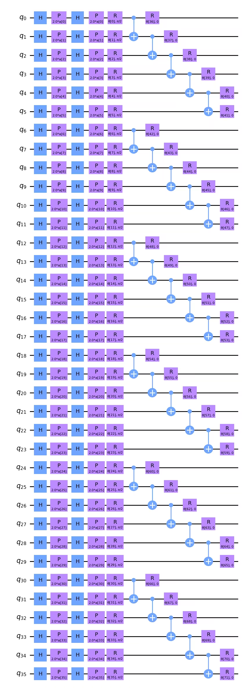
2-Qubit 깊이를 최소화하는 것이 최우선 과제라면, CNOT의 순서를 변경하여 깊이를 약간 줄일 수 있다는 점을 눈치채셨을 것입니다. 예를 들어, 위의 Circuit 다이어그램에서 와 의 CNOT을 왼쪽으로 이동시켜 과 의 CNOT 바로 아래에 배치할 수 있습니다. 2-Qubit 게이트 깊이가 5인 경우, Transpiler 이후에 차이가 생길지는 분명하지 않지만, 염두에 둘 만한 사항입니다. CNOT 게이트의 순서가 다루는 문제의 논리적 구조와 중요하게 맞아야 한다면 현재 깊이로 충분합니다. CNOT의 순서가 이미지의 데이터 구조를 모델링하는 데 중요하지 않다면, 이 CNOT 게이트의 순서를 재배열하여 깊이를 최소화하는 스크립트를 작성할 수도 있습니다.
더 큰 이미지에 맞게 Observable도 재정의해야 합니다:
from qiskit.quantum_info import SparsePauliOp

observable = SparsePauliOp.from_list([("Z" * (num_qubits), 1)])
Qiskit Patterns 2단계: 양자 실행을 위한 문제 최적화
Backend 실행을 위한 Backend를 선택하는 것부터 시작합니다. 여기서는 가장 바쁘지 않은 Backend를 사용합니다.
from qiskit_ibm_runtime import QiskitRuntimeService

# To run on hardware, select the least busy quantum computer or specify a particular one.
service = QiskitRuntimeService()
backend = service.least_busy(operational=True, simulator=False)
# backend = service.backend("ibm_brisbaneane")

print(backend.name)
ibm_brisbane
다시 한번, 최적화 수준을 3으로 설정하여 pass manager를 정의합니다.
from qiskit.circuit.library import XGate
from qiskit.transpiler import PassManager
from qiskit.transpiler.passes import (
    ALAPScheduleAnalysis,
    ConstrainedReschedule,
    PadDynamicalDecoupling,
)
from qiskit.transpiler.preset_passmanagers import generate_preset_pass_manager

target = backend.target

pm = generate_preset_pass_manager(target=target, optimization_level=3)
pm.scheduling = PassManager(
    [
        ALAPScheduleAnalysis(target=target),
        ConstrainedReschedule(
            acquire_alignment=target.acquire_alignment,
            pulse_alignment=target.pulse_alignment,
            target=target,
        ),
        PadDynamicalDecoupling(
            target=target,
            dd_sequence=[XGate(), XGate()],
            pulse_alignment=target.pulse_alignment,
        ),
    ]
)
이제 pass manager를 여러 번 적용합니다. 매우 넓거나 깊은 Circuit의 경우, 트랜스파일된 2-Qubit 깊이에 큰 변동이 있을 수 있습니다. 이러한 Circuit의 경우, pass manager를 여러 번 시도하고 가장 얕은(최선의) 결과를 사용하는 것이 중요합니다.
# Try pass manager several times, since heuristics can return various transpilations on large
# circuits, and we want the shallowest.

transpiled_qcs = []
transpiled_depths = []
transpiled_2q_depths = []
for i in range(1, 10):
    circuit_ibm = pm.run(full_circuit)
    transpiled_qcs.append(circuit_ibm)
    transpiled_depths.append(circuit_ibm.decompose().depth())
    transpiled_2q_depths.append(
        circuit_ibm.decompose().depth(lambda instr: len(instr.qubits) > 1)
    )
    # print(i)

print(transpiled_depths)
print(transpiled_2q_depths)

# Use the shallowest

minpos = transpiled_2q_depths.index(min(transpiled_2q_depths))
[85, 85, 81, 89, 81, 81, 89, 85, 85]
[10, 10, 10, 10, 10, 10, 10, 10, 10]
이 경우, 트랜스파일된 2-Qubit 깊이는 항상 10이었음을 알 수 있습니다. 단일 qubit 깊이에는 약간의 변동이 있었으며, 가장 얕은 것을 사용합니다. 하지만 이 36-Qubit Circuit에서는 이것이 결정적인 개선은 아닙니다. 트랜스파일된 Circuit을 시각화할 수 있지만, 이 규모에서는 시각적으로 파악하기가 점점 어려워집니다.
circuit_ibm = transpiled_qcs[2]
observable_ibm = observable.apply_layout(circuit_ibm.layout)
print(circuit_ibm.decompose().depth())
print(
    f"2+ qubit depth: {circuit_ibm.decompose().depth(lambda instr: len(instr.qubits) > 1)}"
)
81
2+ qubit depth: 10
Qiskit Patterns 3단계: Qiskit Primitives를 사용한 실행
실제 양자 컴퓨터에서 사용되는 시간을 제한하기 위해, 여기서는 최적화 단계를 몇 번만 수행하며 매우 작은 훈련 데이터셋을 사용합니다. 하지만 더 많은 최적화 단계와 더 큰 테스트 데이터셋으로의 확장은 이 레슨 전반에 걸친 지침에서 명확하게 설명됩니다.
# This was run on an Eagle r3 processor on 10-4-24, and took 7 min.

from qiskit_ibm_runtime import EstimatorV2 as Estimator, Session

batch_size = 7
num_epochs = 1
num_samples = len(train_images)

# Globals
circuit = circuit_ibm
observable = observable_ibm
objective_func_vals = []
iter = 0

# Random initial weights for the ansatz
np.random.seed(42)
# weight_params = np.random.rand(len(ansatz.parameters)) * 2 * np.pi
# Or re-load weights from a previous calculation
weight_params = np.array(
    [
        3.35330497,
        5.97351416,
        4.59925358,
        3.76148219,
        0.98029403,
        0.98014248,
        0.3649501,
        6.44234523,
        3.77691701,
        4.44895122,
        0.12933619,
        6.09412333,
        5.23039137,
        1.33416598,
        1.14243996,
        1.15236452,
        1.91161039,
        3.2971419,
        3.71399059,
        1.82984665,
        3.84438512,
        0.87646578,
        1.83559896,
        2.30191935,
        2.86557222,
        4.93340606,
        1.25458737,
        3.23103027,
        3.72225051,
        0.29185655,
        3.81731689,
        1.07143467,
        0.40873121,
        5.96202367,
        6.067245,
        5.07931034,
        1.91394476,
        0.61369199,
        4.2991629,
        2.76555968,
        0.76678884,
        3.11128829,
        0.21606945,
        5.71342859,
        1.62596258,
        4.16275028,
        1.95853845,
        3.26768375,
        3.43508199,
        1.1614748,
        6.09207989,
        4.87030317,
        5.90304595,
        5.62236606,
        3.75671636,
        5.79230665,
        0.55601479,
        1.23139664,
        0.28417144,
        2.04411075,
        2.44213144,
        1.70493625,
        5.20711134,
        2.24154726,
        1.76516358,
        3.40986006,
        0.88545302,
        5.04035228,
        0.46841551,
        6.2007935,
        4.85215699,
        1.24856745,
    ]
)

# Running in a session avoids repeated queuing. This is available to Premium Plan, Flex Plan, and
# On-Prem (IBM Quantum Platform API) Plan users.

with Session(backend=backend) as session:
    estimator = Estimator(mode=session, options={"resilience_level": 1})

    for epoch in range(num_epochs):
        for i in range((num_samples - 1) // batch_size + 1):
            print(f"Epoch: {epoch}, batch: {i}")
            start_i = i * batch_size
            end_i = start_i + batch_size
            train_images_batch = np.array(train_images[start_i:end_i])
            train_labels_batch = np.array(train_labels[start_i:end_i])
            input_params = train_images_batch
            target = train_labels_batch
            iter = 0
            # We can increase maxiter to do a full optimization.
            res = minimize(
                mse_loss_weights,
                weight_params,
                method="COBYLA",
                options={"maxiter": 20},
            )
            weight_params = res["x"]
session.close()

# Open users can carry out the same calculation using a batch, but repeated queuing is possible.
# from qiskit_ibm_runtime import Batch

# with Batch(backend=backend) as batch:
#    estimator = Estimator(
#        mode=batch, options={"resilience_level": 1}
#    )
#
#    for epoch in range(num_epochs):
#        for i in range((num_samples - 1) // batch_size + 1):
#            print(f"Epoch: {epoch}, batch: {i}")
#            start_i = i * batch_size
#            end_i = start_i + batch_size
#            train_images_batch = np.array(train_images[start_i:end_i])
#            train_labels_batch = np.array(train_labels[start_i:end_i])
#            input_params = train_images_batch
#            target = train_labels_batch
#            iter = 0
#            # We can increase maxiter to do a full optimization.
#            res = minimize(
#                mse_loss_weights,
#                weight_params,
#                method="COBYLA",
#                options={"maxiter": 20},
#            )
#            weight_params = res["x"]
# batch.close()
이 계산에서 반환된 가중치 파라미터를 저장해 두는 것을 권장합니다. 추후 반복 계산을 진행하고자 할 때 유용합니다.
weight_params
array([3.35330497, 6.97351416, 5.59925358, 3.76148219, 0.98029403,
       0.98014248, 0.3649501 , 6.44234523, 3.77691701, 4.44895122,
       1.12933619, 7.09412333, 5.23039137, 1.33416598, 1.14243996,
       1.15236452, 1.91161039, 3.2971419 , 3.71399059, 1.82984665,
       3.84438512, 0.87646578, 1.83559896, 2.30191935, 2.86557222,
       4.93340606, 1.25458737, 3.23103027, 3.72225051, 0.29185655,
       3.81731689, 1.07143467, 0.40873121, 5.96202367, 6.067245  ,
       5.07931034, 1.91394476, 0.61369199, 4.2991629 , 2.76555968,
       0.76678884, 3.11128829, 0.21606945, 5.71342859, 1.62596258,
       4.16275028, 1.95853845, 3.26768375, 3.43508199, 1.1614748 ,
       6.09207989, 4.87030317, 5.90304595, 5.62236606, 3.75671636,
       5.79230665, 0.55601479, 1.23139664, 0.28417144, 2.04411075,
       2.44213144, 1.70493625, 5.20711134, 2.24154726, 1.76516358,
       3.40986006, 0.88545302, 5.04035228, 0.46841551, 6.2007935 ,
       4.85215699, 1.24856745])
처음 몇 번의 최적화 단계를 플롯할 수 있지만, 단 몇 단계만으로는 수렴을 기대할 수 없습니다. 시뮬레이터를 사용하더라도 처음 몇 단계에서는 이 곡선들이 비교적 평탄한 경향을 보였습니다. 그러나 현재 최적화에는 72개의 자유 파라미터가 있다는 점을 주목해야 합니다. 예를 들어, 전체 행과 열의 일부 데이터에 해당하는 Qubit를 파라미터화하는 방식으로 결과를 저하시키지 않고 파라미터 공간을 최소 2~3배 줄일 수 있습니다. 실제로 손실 함수를 최소화하는 데 더 많은 양자 컴퓨팅 시간을 투자하기 전에 파라미터 공간을 줄여야 합니다.
obj_func_vals_qc = objective_func_vals
# import matplotlib.pyplot as plt

plt.figure(figsize=(12, 6))
plt.plot(obj_func_vals_qc, label="revised ansatz")
plt.xlabel("iteration")
plt.ylabel("loss")
plt.legend()
plt.show()

마무리
요약하자면, 이 레슨에서는 양자 신경망을 사용한 이미지 이진 분류 워크플로를 학습했습니다. 각 Qiskit Patterns 단계에서의 주요 고려 사항은 다음과 같습니다:
Step 1: 문제를 양자 Circuit으로 매핑하기
- 훈련 데이터를 로드합니다. 이는 "수동으로" 하거나
z_feature_map과 같은 사전 구축된 feature map을 사용해서 할 수 있습니다. - 문제에 적합한 회전 및 얽힘 레이어를 포함하는 ansatz를 구성합니다.
- 양자 컴퓨터에서 품질 높은 결과를 보장하기 위해 Circuit 깊이를 모니터링합니다.
Step 2: 양자 실행을 위한 문제 최적화
- Backend를 선택합니다. 보통 가장 바쁘지 않은 것을 선택합니다.
- pass manager를 사용하여 Circuit과 Observable을 선택한 Backend의 아키텍처에 맞게 트랜스파일합니다.
- 매우 깊거나 넓은 Circuit의 경우, 여러 번 트랜스파일하고 가장 얕은 Circuit을 선택합니다.
Step 3: Qiskit (Runtime) Primitives를 사용하여 실행하기
- 시뮬레이터에서 예비 시험을 수행하여 ansatz를 디버그하고 최적화합니다.
- IBM® 양자 컴퓨터에서 실행합니다.
Step 4: 후처리, 고전적 형식으로 결과 반환하기
- 훈련 데이터와 테스트 데이터에 대한 모델 정확도를 계산합니다.
- 고전적 최적화의 수렴을 모니터링합니다.