연산자 역전파를 이용한 회로 깊이 감소

연산자 역전파(operator backpropagation)는 양자 회로의 끝단에 있는 연산들을 Pauli 연산자 속으로 흡수시키는 기법으로, 일반적으로 연산자의 항 수가 늘어나는 비용을 치르고 회로의 깊이를 줄입니다. 목표는 연산자가 지나치게 커지지 않도록 하면서 가능한 한 많이 회로를 역전파하는 것입니다.

연산자가 지나치게 커지지 않도록 하면서 회로에 대해 더 깊이 역전파하도록 허용하는 한 가지 방법은, 계수가 작은 항들을 연산자에 추가하는 대신 잘라내는(truncation) 것입니다. 항을 잘라내면 실행해야 할 양자 회로의 수가 줄어들 수 있지만, 그렇게 하면 잘라낸 항들의 계수 크기에 비례한 오차가 최종 기댓값 계산에 생깁니다. 이 튜토리얼에서는 연산자 역전파를 사용하여 Heisenberg 스핀 체인의 양자 동역학을 시뮬레이션하는 Qiskit 패턴을 구현합니다:

• 1단계: 양자 문제로 매핑
  • 시간 변화 Hamiltonian을 양자 회로에 매핑합니다
• 2단계: 문제 최적화
  • 회로를 슬라이스합니다
  • 회로의 슬라이스들을 Pauli observable로 역전파합니다
  • 남은 슬라이스들을 단일 회로로 결합합니다
  • 회로를 backend용으로 transpile합니다
• 3단계: 실험 실행
  • 이 노트북에서는 간단하게 하기 위해 StatevectorEstimator를 사용하여 축소된 회로와 확장된 observable로 기댓값을 계산합니다
• 4단계: 결과 재구성
  • 해당 없음

참고: Qiskit은 layer를 모든 qubit에 걸친 회로의 깊이 1짜리 파티션이라고 느슨하게 표현합니다. 이 패키지는 임의 깊이의 레이어를 설명하기 위해 **슬라이스(slices)**라는 용어를 사용합니다. qiskit_addon_obp.backpropagate 함수는 한 번에 전체 슬라이스를 역전파하도록 설계되어 있으므로, 양자 회로를 어떻게 슬라이스할지에 대한 선택은 주어진 문제에 대해 역전파가 얼마나 잘 수행되는지에 큰 영향을 미칠 수 있습니다. 아래에서 슬라이스에 대해 더 자세히 알게 될 것입니다.

1단계: 양자 문제로 매핑

양자 Heisenberg 모델의 시간 변화를 양자 실험으로 매핑합니다.

qiskit_addon_utils 패키지는 다양한 용도로 재사용 가능한 기능들을 제공합니다.

이 패키지의 qiskit_addon_utils.problem_generators 모듈은 주어진 연결 그래프 위에서 Heisenberg 유사 Hamiltonian을 생성하는 함수를 제공합니다. 이 그래프는 rustworkx.PyGraph 또는 CouplingMap일 수 있으므로, Qiskit 중심의 워크플로우에서 쉽게 사용할 수 있습니다.

다음에서는 먼저 heavy-hex CouplingMap을 생성한 뒤, 여기서 10개의 qubit으로 이루어진 선형 체인을 잘라냅니다. 이 새로운 reduced_coupling_map의 인덱스는 다시 0부터 시작한다는 점에 유의하세요.

# Added by doQumentation — required packages for this notebook
!pip install -q numpy qiskit qiskit-addon-obp qiskit-addon-utils qiskit-ibm-runtime rustworkx

from qiskit.transpiler import CouplingMap

coupling_map = CouplingMap.from_heavy_hex(3, bidirectional=False)

# Choose a 10-qubit linear chain on this coupling map
reduced_coupling_map = coupling_map.reduce([0, 13, 1, 14, 10, 16, 5, 12, 8, 18])

from rustworkx.visualization import graphviz_draw

graphviz_draw(reduced_coupling_map.graph, method="circo")

다음으로, Heisenberg XYZ Hamiltonian을 모델링하는 Pauli 연산자를 생성합니다.

J_{y} \sigma_j^{y} \sigma_{k}^{y} + J_{z} \sigma_j^{z} \sigma_{k}^{z}) + \sum_{j\in V} (h_{x} \sigma_j^{x} + h_{y} \sigma_j^{y} + h_{z} \sigma_j^{z})$$ 여기서 $G(V,E)$는 제공된 coupling map의 그래프입니다. ```python import numpy as np from qiskit_addon_utils.problem_generators import generate_xyz_hamiltonian # Get a qubit operator describing the Heisenberg XYZ model hamiltonian = generate_xyz_hamiltonian( reduced_coupling_map, coupling_constants=(np.pi / 8, np.pi / 4, np.pi / 2), ext_magnetic_field=(np.pi / 3, np.pi / 6, np.pi / 9), ) print(hamiltonian) ``` ```text SparsePauliOp(['IIIIIIIXXI', 'IIIIIIIYYI', 'IIIIIIIZZI', 'IIIIIXXIII', 'IIIIIYYIII', 'IIIIIZZIII', 'IIIXXIIIII', 'IIIYYIIIII', 'IIIZZIIIII', 'IXXIIIIIII', 'IYYIIIIIII', 'IZZIIIIIII', 'IIIIIIIIXX', 'IIIIIIIIYY', 'IIIIIIIIZZ', 'IIIIIIXXII', 'IIIIIIYYII', 'IIIIIIZZII', 'IIIIXXIIII', 'IIIIYYIIII', 'IIIIZZIIII', 'IIXXIIIIII', 'IIYYIIIIII', 'IIZZIIIIII', 'XXIIIIIIII', 'YYIIIIIIII', 'ZZIIIIIIII', 'IIIIIIIIIX', 'IIIIIIIIIY', 'IIIIIIIIIZ', 'IIIIIIIIXI', 'IIIIIIIIYI', 'IIIIIIIIZI', 'IIIIIIIXII', 'IIIIIIIYII', 'IIIIIIIZII', 'IIIIIIXIII', 'IIIIIIYIII', 'IIIIIIZIII', 'IIIIIXIIII', 'IIIIIYIIII', 'IIIIIZIIII', 'IIIIXIIIII', 'IIIIYIIIII', 'IIIIZIIIII', 'IIIXIIIIII', 'IIIYIIIIII', 'IIIZIIIIII', 'IIXIIIIIII', 'IIYIIIIIII', 'IIZIIIIIII', 'IXIIIIIIII', 'IYIIIIIIII', 'IZIIIIIIII', 'XIIIIIIIII', 'YIIIIIIIII', 'ZIIIIIIIII'], coeffs=[0.39269908+0.j, 0.78539816+0.j, 1.57079633+0.j, 0.39269908+0.j, 0.78539816+0.j, 1.57079633+0.j, 0.39269908+0.j, 0.78539816+0.j, 1.57079633+0.j, 0.39269908+0.j, 0.78539816+0.j, 1.57079633+0.j, 0.39269908+0.j, 0.78539816+0.j, 1.57079633+0.j, 0.39269908+0.j, 0.78539816+0.j, 1.57079633+0.j, 0.39269908+0.j, 0.78539816+0.j, 1.57079633+0.j, 0.39269908+0.j, 0.78539816+0.j, 1.57079633+0.j, 0.39269908+0.j, 0.78539816+0.j, 1.57079633+0.j, 1.04719755+0.j, 0.52359878+0.j, 0.34906585+0.j, 1.04719755+0.j, 0.52359878+0.j, 0.34906585+0.j, 1.04719755+0.j, 0.52359878+0.j, 0.34906585+0.j, 1.04719755+0.j, 0.52359878+0.j, 0.34906585+0.j, 1.04719755+0.j, 0.52359878+0.j, 0.34906585+0.j, 1.04719755+0.j, 0.52359878+0.j, 0.34906585+0.j, 1.04719755+0.j, 0.52359878+0.j, 0.34906585+0.j, 1.04719755+0.j, 0.52359878+0.j, 0.34906585+0.j, 1.04719755+0.j, 0.52359878+0.j, 0.34906585+0.j, 1.04719755+0.j, 0.52359878+0.j, 0.34906585+0.j]) ``` qubit 연산자로부터 그 시간 변화를 모델링하는 양자 회로를 생성할 수 있습니다. 다시 한 번, [qiskit_addon_utils.problem_generators](https://qiskit.github.io/qiskit-addon-utils/stubs/qiskit_addon_utils.problem_generators.html) 모듈이 편리한 함수를 통해 바로 그 작업을 해결해 줍니다: ```python from qiskit.synthesis import LieTrotter from qiskit_addon_utils.problem_generators import generate_time_evolution_circuit circuit = generate_time_evolution_circuit( hamiltonian, time=0.2, synthesis=LieTrotter(reps=2), ) circuit.draw("mpl", style="iqp", scale=0.6) ``` 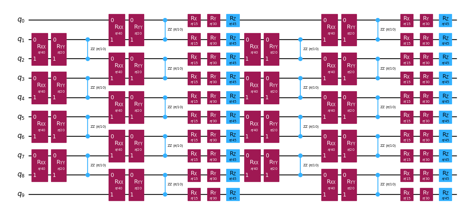 ## 2단계: 문제 최적화 \{#step-2-optimize-the-problem} ### 역전파할 회로 슬라이스 생성 \{#create-circuit-slices-to-backpropagate} ``backpropagate`` 함수는 한 번에 전체 회로 슬라이스를 역전파한다는 점을 기억하세요. 따라서 슬라이스를 어떻게 나누는지에 대한 선택은 주어진 문제에서 역전파가 얼마나 잘 수행되는지에 영향을 줄 수 있습니다. 여기서는 [slice_by_gate_types](https://qiskit.github.io/qiskit-addon-utils/stubs/qiskit_addon_utils.slicing.slice_by_gate_types.html) 함수를 사용하여 같은 타입의 Gate들을 하나의 슬라이스로 묶겠습니다. 회로 슬라이싱에 대한 더 자세한 논의는 [qiskit-addon-utils](https://qiskit.github.io/qiskit-addon-utils/index.html) 패키지의 [how-to 가이드](https://qiskit.github.io/qiskit-addon-utils/how_tos/create_circuit_slices.html)를 참조하세요. ```python from qiskit_addon_utils.slicing import slice_by_gate_types slices = slice_by_gate_types(circuit) print(f"Separated the circuit into {len(slices)} slices.") ``` ```text Separated the circuit into 18 slices. ``` ### 역전파 중 연산자가 얼마나 커질 수 있는지 제한하기 \{#constrain-how-large-the-operator-may-grow-during-backpropagation} 역전파가 진행되는 동안, 연산자의 항 수는 일반적으로 빠르게 $4^N$에 가까워집니다. 여기서 $N$은 qubit 수입니다. 연산자의 크기는 ``backpropagate`` 함수의 ``operator_budget`` kwarg를 지정하여 제한할 수 있으며, 이는 [OperatorBudget](https://qiskit.github.io/qiskit-addon-obp/stubs/qiskit_addon_obp.utils.simplify.OperatorBudget.html) 인스턴스를 받습니다. 여기서는 연산자 내 qubit별 가환(qubit-wise commuting) Pauli 그룹의 수가 8을 초과할 때 역전파를 중단하도록 지정합니다. ```python from qiskit_addon_obp.utils.simplify import OperatorBudget op_budget = OperatorBudget(max_qwc_groups=8) ``` ### 회로의 슬라이스들을 역전파하기 \{#backpropagate-slices-from-the-circuit} 먼저, qubit 0에 대한 Pauli-Z observable을 지정하고, observable의 항들이 더 이상 8개 이하의 qubit별 가환 Pauli 그룹으로 결합될 수 없을 때까지 시간 변화 회로의 슬라이스들을 역전파합니다. 아래에서 보듯이 7개의 슬라이스를 역전파했지만 할당된 8개의 Pauli 그룹 중 6개만 사용했습니다. 이는 슬라이스를 하나 더 역전파하면 Pauli 그룹 수가 8을 초과함을 의미합니다. 반환된 메타데이터를 조사하여 이를 확인할 수 있습니다. ```python from qiskit.quantum_info import SparsePauliOp from qiskit_addon_obp import backpropagate from qiskit_addon_utils.slicing import combine_slices # Specify a single-qubit observable observable = SparsePauliOp("IIIIIIIIIZ") # Backpropagate slices onto the observable bp_obs, remaining_slices, metadata = backpropagate(observable, slices, operator_budget=op_budget) # Recombine the slices remaining after backpropagation bp_circuit = combine_slices(remaining_slices, include_barriers=True) print(f"Backpropagated {metadata.num_backpropagated_slices} slices.") print( f"New observable has {len(bp_obs.paulis)} terms, which can be combined into {len(bp_obs.group_commuting(qubit_wise=True))} groups." ) print( f"Note that backpropagating one more slice would result in {metadata.backpropagation_history[-1].num_paulis[0]} terms " f"across {metadata.backpropagation_history[-1].num_qwc_groups} groups." ) print("The remaining circuit after backpropagation looks as follows:") bp_circuit.draw("mpl", scale=0.6) ``` ```text Backpropagated 7 slices. New observable has 18 terms, which can be combined into 8 groups. Note that backpropagating one more slice would result in 27 terms across 12 groups. The remaining circuit after backpropagation looks as follows: ``` 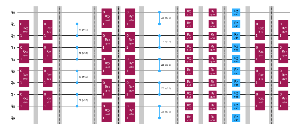 다음으로, 출력 observable 크기에 대한 동일한 제약으로 동일한 문제를 지정하겠습니다. 그러나 이번에는 [setup_budet](https://qiskit.github.io/qiskit-addon-obp/stubs/qiskit_addon_obp.utils.truncating.setup_budget.html) 함수를 사용하여 각 슬라이스에 오차 예산(error budget)을 할당합니다. 각 슬라이스에서 작은 계수를 가진 Pauli 항들은 오차 예산이 채워질 때까지 잘려나가며, 남은 예산은 다음 슬라이스의 예산에 더해집니다. 이 절단(truncation)을 활성화하려면 오차 예산을 다음과 같이 설정해야 합니다: ```python from qiskit_addon_obp.utils.truncating import setup_budget truncation_error_budget = setup_budget(max_error_per_slice=0.005) ``` 슬라이스당 `5e-3`의 오차를 절단에 할당함으로써, observable 내 가환 Pauli 그룹 8개의 원래 예산을 유지하면서도 회로에서 슬라이스를 3개 더 제거할 수 있다는 점에 주목하세요. 기본적으로 `backpropagate`는 절단으로 인한 총 오차를 제한하기 위해 잘라낸 계수들의 L1 노름을 사용합니다. 다른 옵션에 대해서는 [p_norm 지정에 대한 how-to 가이드](https://qiskit.github.io/qiskit-addon-obp/how_tos/bound_error_using_p_norm.html)를 참조하세요. 10개의 슬라이스를 역전파한 이 특정 예제에서는 총 절단 오차가 ``(5e-3 error/slice) * (10 slices) = 5e-2``를 초과하지 않아야 합니다. 슬라이스들에 오차 예산을 분배하는 것에 대한 추가 논의는 [이 how-to 가이드](https://qiskit.github.io/qiskit-addon-obp/how_tos/truncate_operator_terms.html)를 참조하세요. ```python # Run the same experiment but truncate observable terms with small coefficients bp_obs_trunc, remaining_slices_trunc, metadata = backpropagate( observable, slices, operator_budget=op_budget, truncation_error_budget=truncation_error_budget ) # Recombine the slices remaining after backpropagation bp_circuit_trunc = combine_slices(remaining_slices_trunc, include_barriers=True) print(f"Backpropagated {metadata.num_backpropagated_slices} slices.") print( f"New observable has {len(bp_obs_trunc.paulis)} terms, which can be combined into {len(bp_obs_trunc.group_commuting(qubit_wise=True))} groups.\n" f"After truncation, the error in our observable is bounded by {metadata.accumulated_error(0):.3e}" ) print( f"Note that backpropagating one more slice would result in {metadata.backpropagation_history[-1].num_paulis[0]} terms " f"across {metadata.backpropagation_history[-1].num_qwc_groups} groups." ) print("The remaining circuit after backpropagation looks as follows:") bp_circuit_trunc.draw("mpl", scale=0.6) ``` ```text Backpropagated 10 slices. New observable has 19 terms, which can be combined into 8 groups. After truncation, the error in our observable is bounded by 4.933e-02 Note that backpropagating one more slice would result in 27 terms across 13 groups. The remaining circuit after backpropagation looks as follows: ``` 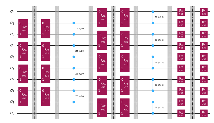 ### 이제 축소된 ansatz와 확장된 observable을 얻었으므로, 실험을 backend용으로 transpile할 수 있습니다. \{#now-that-we-have-our-reduced-ansatze-and-expanded-observables-we-can-transpile-our-experiments-to-the-backend} 여기서는 [qiskit-ibm-runtime](https://quantum.cloud.ibm.com/docs/api/qiskit-ibm-runtime)의 14-qubit [FakeMelbourneV2](https://quantum.cloud.ibm.com/docs/api/qiskit-ibm-runtime/fake-provider-fake-melbourne-v2)를 사용하여 QPU backend로 transpile하는 방법을 시연합니다. ```python from qiskit.transpiler.preset_passmanagers import generate_preset_pass_manager from qiskit_ibm_runtime.fake_provider import FakeMelbourneV2 # Specify a backend and a pass manager for transpilation backend = FakeMelbourneV2() pm = generate_preset_pass_manager(backend=backend, optimization_level=1) # Transpile original experiment circuit_isa = pm.run(circuit) observable_isa = observable.apply_layout(circuit_isa.layout) # Transpile backpropagated experiment bp_circuit_isa = pm.run(bp_circuit) bp_obs_isa = bp_obs.apply_layout(bp_circuit_isa.layout) # Transpile the backpropagated experiment with truncated observable terms bp_circuit_trunc_isa = pm.run(bp_circuit_trunc) bp_obs_trunc_isa = bp_obs_trunc.apply_layout(bp_circuit_trunc_isa.layout) ``` ## 3단계: 양자 실험 실행 \{#step-3-execute-quantum-experiments} ### 기댓값 계산 \{#calculate-expectation-value} 마지막으로, 노이즈 없는 [StatevectorEstimator](https://quantum.cloud.ibm.com/docs/api/qiskit/qiskit.primitives.StatevectorEstimator)를 사용하여 역전파된 실험을 실행하고 전체 실험과 비교할 수 있습니다. 절단 없이 역전파된 기댓값은 수치 정밀도 한계 내에서 정확한 값과 동일함을 확인할 수 있습니다. 절단된 항이 있는 연산자에 대한 기댓값은 ``1e-4`` 수준의 일부 오차를 가지며, 이는 예상 허용 오차 범위 내에 있습니다. **참고:** 출력에 미치는 절단의 영향을 보이기 위해 statevector 기반의 ``Estimator`` 프리미티브를 사용합니다. 2단계에서 실험을 transpile한 backend에서 실행하려면, ``qiskit-ibm-runtime``에서 [EstimatorV2](https://quantum.cloud.ibm.com/docs/api/qiskit-ibm-runtime/estimator-v2)를 import하여 생성자에 backend 인스턴스를 전달하면 됩니다. ```python from qiskit.primitives import StatevectorEstimator as Estimator estimator = Estimator() # Run the experiments using Estimator primitive result_exact = estimator.run([(circuit_isa, observable_isa)]).result()[0].data.evs.item() result_bp = estimator.run([(bp_circuit_isa, bp_obs_isa)]).result()[0].data.evs.item() result_bp_trunc = ( estimator.run([(bp_circuit_trunc_isa, bp_obs_trunc_isa)]).result()[0].data.evs.item() ) print(f"Exact expectation value: {result_exact}") print(f"Backpropagated expectation value: {result_bp}") print(f"Backpropagated expectation value with truncation: {result_bp_trunc}") print(f" - Expected Error for truncated observable: {metadata.accumulated_error(0):.3e}") print(f" - Observed Error for truncated observable: {abs(result_exact - result_bp_trunc):.3e}") ``` ```text Exact expectation value: 0.8854160687717507 Backpropagated expectation value: 0.8854160687717532 Backpropagated expectation value with truncation: 0.8850236647156059 - Expected Error for truncated observable: 4.933e-02 - Observed Error for truncated observable: 3.924e-04 ``` <TutorialFeedback />