음영 라이트콘을 활용한 확률적 오류 소거
배경
이 튜토리얼에서는 음영 라이트콘(SLC) 애드온을 사용해 오류를 완화하는 방법을 보여줘요. 이 애드온은 확률적 오류 소거(PEC) 기법의 발전된 형태로, 사용자가 회로의 고유한 레이어에 대한 노이즈를 학습한 다음 단일 큐비트 게이트와 후처리 기법을 적용해 노이즈를 소거해요. 다른 방법과 비교할 때 PEC는 완화된 결과의 편향에 대해 더 강력한 경계를 제공하지만, QPU 시간 측면에서 더 높은 오버헤드를 갖는 경향이 있어요. PEC에서는 노이즈에 의한 기댓값 감쇠를 보상하기 위해 평균 결과를 인수로 재조정해요. 여기서 는 회로의 레이어 에서 오류 Pauli 의 학습된 노이즈 율이에요. 이 재조정은 분산을 배 증가시키며, 따라서 QPU에서 필요한 회로 실행 횟수도 배 곱해져요. 이를 샘플링 비용 또는 샘플링 오버헤드라고 해요. 는 지수적으로 증가하기 때문에 PEC는 얕거나 소수의 큐비트로 구성된 회로에 제한되는 경우가 많아요. PEC에 대한 자세한 내용은 Probabilistic error cancellation with sparse Pauli-Lindblad models on noisy quantum processors를 참조하세요.
완화할 필요가 없는 오류를 식별할 수 있다면, 이 샘플링 비용을 지수적으로 줄일 수 있어요. 이 방향의 첫 번째 단계는 로컬 인식 오류 완화를 구현하는 것이에요. 이는 빠르게 계산 가능한 기존 "라이트콘"을 사용해 회로 전체에 걸친 관측량의 오류 민감도를 경계짓는 방식으로 PEC 오버헤드를 줄여, 일부 문제에서 PEC의 적용 가능 규모를 확장해요. 이 라이트콘 밖에 있는 오류는 측정 결과에 영향을 미칠 수 없으므로 오류 소거 절차에서 제외할 수 있어요. 이 제외는 추가적인 편향을 도입하지 않으면서 경우에 따라 상당한 수준으로 샘플링 오버헤드를 줄여요. 특히, 고정 깊이 회로에서 로컬 관측량 를 측정할 때, 필요한 샘플링 오버헤드는 회로의 큐비트 수를 늘려도 결국 평탄해져요(Locality and Error Mitigation of Quantum Circuits의 Fig. 2b 참조).
음영 라이트콘(SLC)은 한 단계 더 나아가 고전 시뮬레이션을 사용해 회로 전체에 걸친 오류 민감도를 더 엄밀하게 경계짓어요. 이는 일부 QPU 시간을 CPU 시간으로 대체하고, 편향을 재정규화하는 데 필요한 샘플링 오버헤드를 줄여요. 경계가 명확히 잘리는 것이 아니라 회로 내의 각 잠재적 오류에 대해 관측량의 해당 오류에 대한 민감도의 상한을 나타내는 단계적 "음영"이 부여돼요. 이 정밀한 특성 분석은 감소된 분산으로 더 효율적이고 표적화된 PEC 적용을 할 수 있게 하는 동시에 사용자가 관측량 추정의 편향을 조절해서 조정할 수 있게 해요. 자세한 내용은 Lightcone shading for classically accelerated quantum error mitigation을 참조하세요.
SLC 애드온을 위한 워크플로우는 새로운 Samplomatic 및 Executor 프레임워크를 활용하여, 고급 사용자에게는 사용 편의성을 유지하면서 오류 억제 및 완화를 위한 실행 설정에 대한 모듈식 제어를 제공합니다. 이 프레임워크의 이점과 일반적인 기능에 대한 더 깊은 이해를 위해 Hello samplomatic 튜토리얼을 참조하세요.
라이트콘 음영, 노이즈 학습, 안티노이즈 주입 워크플로우
QPU의 노이즈를 모델링하기 위해, 장치의 각 큐비트 및 엣지에서 로컬로 생성된 1- 및 2-큐비트 Pauli 오류율을 갖는 희소 Pauli-Lindblad 노이즈 모델을 사용하기로 했습니다. 이 선택을 통해 이 튜토리얼에서 제시하는 SLC 오류 완화 워크플로우는 다음과 같습니다:
a. CPU — 1- 및 2-큐비트 Pauli 오류의 오류당 영향 경계 산정
-
순방향 전파(관측량에 대한 영향 경계). 각 오류를 회로의 끝까지 전파하고 관측량과의 교환자를 계산합니다.
-
계산량을 감당 가능한 수준으로 유지하기 위해 진화 중 연산자 항을 잘라내요.
-
양자 속도 한계에 기반한 느슨한 역방향 전파로 이 경계를 더욱 조입니다.
-
-
역방향 전파(초기 상태에 대한 영향 경계). 각 오류를 회로의 시작 부분까지 전파하고 초기 상태와의 교환자를 계산합니다.
b. QPU — 노이즈 율 학습. NoiseLearner를 사용해 Pauli-Lindblad 노이즈 모델의 율을 추정해요.
c. CPU — 완화 우선순위 지정
-
학습된 노이즈 율로 병합 경계 업데이트. 이전에 계산된 순방향 및 역방향 경계를 결합하고 학습된 노이즈 율로 업데이트합니다.
-
계산된 경계와 학습된 율을 사용해 완화할 노이즈 구성 요소의 순위를 지정해요. 편향에 대한 추정 영향과 수정에 드는 비용을 기반으로 각 가능한 노이즈 오류의 우선순위를 정해요.
d. QPU — 안티노이즈 삽입 및 실행. Box 어노테이션을 사용해 지정된 안티노이즈(역 노이즈)로 관심 회로를 실행해요.
e. CPU — 관측량 추정. 비-Markovian 노이즈 영향을 줄이기 위해 측정 기반 후선택을 적용하여 기댓값을 계산합니다.
노이즈 학습 개요
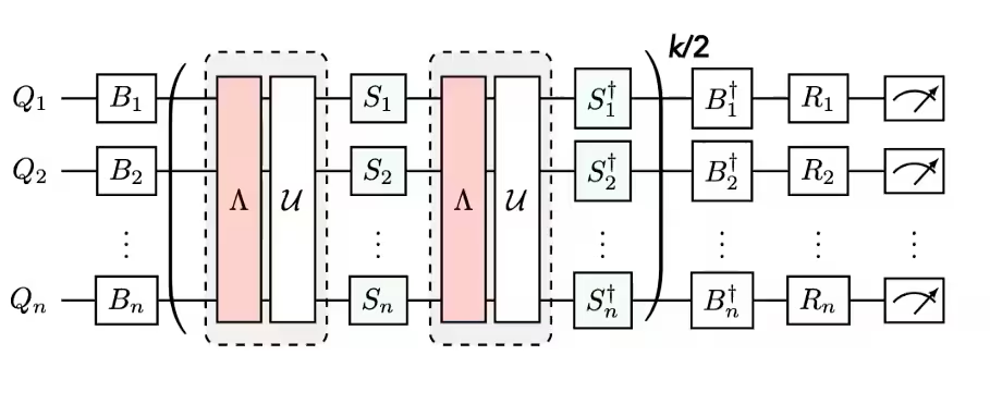
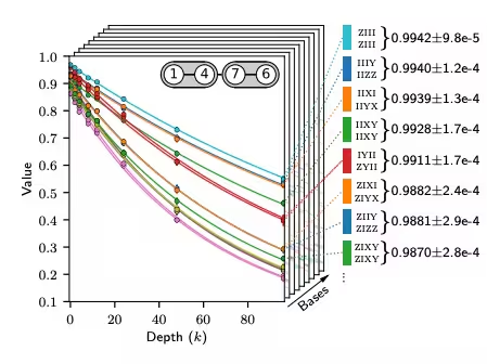
노이즈 학습은 여러 오류 완화 방법에서 공통적인 단계로, NoiseLearner에 의해 수행되며, PEA 오류 완화 튜토리얼과 전파된 노이즈 흡수(PNA) 튜토리얼에서도 확인할 수 있어요. NoiseLearnerV3에서 사용자는 학습할 노이즈 레이어를 CircuitInstruction 객체로 명시적으로 식별할 수 있어, 위에서 설명한 방식으로 각 레이어에 대한 원하는 SLC 노이즈 경계를 계산할 수 있어요. 학습된 Pauli-Lindblad 모델은 PEC-SLC 우선순위 지정에 사용될 계수를 제공해요. 게이트가 레이어로 수집되는 방식은 generate_boxing_pass_manager와 unique_2q_instructions 편의 함수를 사용해 결정한 다음, 아래 2단계에 설명된 대로 SLC 유틸리티 함수 generate_noise_model_paulis에 공급할 수 있어요.
| 파트 1 | 파트 2 | 파트 3 |
|---|---|---|
| 2-큐비트 게이트 레이어 Pauli 트월링 | 레이어의 항등 쌍을 반복하고 노이즈 학습 | 충실도 도출(각 노이즈 채널의 오류) |
 |  |  |
후처리 개요
Samplomatic 및 Executor 프레임워크를 사용해 양자 하드웨어에서 실행한 후, 비트스트링 측정값을 원하는 관측량 값으로 변환해요. 미러링된 Ising 회로의 경우, 모든 큐비트가 이상적으로 시작점인 으로 돌아와야 하므로 측정된 관측량은 이상적으로 1이 되어야 해요. expectation_values 함수로 관측량 값을 계산할 때, 노이즈 영향을 줄이는 몇 가지 후처리 기법을 적용해요. 여기에는 비-Markovian 노이즈의 영향을 받은 샷 제거, 판독 오류 완화, 그리고 PEC 구현의 세부 사항 고려가 포함돼요. 세부 사항은 아래 4단계에서 다뤄요.
요구 사항
이 튜토리얼을 시작하기 전에 다음 패키지가 설치되어 있는지 확인하세요:
-
Executor 프리미티브가 포함된 Qiskit IBM Runtime (
pip install "qiskit-ibm-runtime @ git+https://github.com/Qiskit/qiskit-ibm-runtime.git") -
Qiskit addon Shaded lightcone 0.1 (
pip install "qiskit-addon-slc~=0.1.0") -
Qiskit addon utils (
pip install "qiskit-addon-utils~=0.3.0") -
Samplomatic v0.16 이상 (
pip install samplomatic) -
Qiskit 시각화 지원 (
pip install "qiskit[visualization]")
Step 0. 설정
먼저 이 노트북을 성공적으로 실행하는 데 필요한 패키지와 함수를 가져옵니다.
# Added by doQumentation — installs the packages this notebook needs if they are missing
import importlib.util

_needed = {"matplotlib": "matplotlib", "numpy": "numpy", "qiskit": "qiskit", "qiskit_addon_slc": "qiskit-addon-slc", "qiskit_addon_utils": "qiskit-addon-utils", "qiskit_ibm_runtime": "qiskit-ibm-runtime@git+https://github.com/Qiskit/qiskit-ibm-runtime.git", "samplomatic": "samplomatic"}
_missing = [pip for module, pip in _needed.items()
            if importlib.util.find_spec(module) is None]
# One at a time, so a package that fails to install does not block the others
for _pip in _missing:
    %pip install -q {_pip}
if not _missing:
    print("\u2713 All required packages are installed")
import logging

logging.basicConfig(level=logging.INFO, format="%(asctime)s %(levelname)s %(module)s %(message)s")

# Setting this value prevents itertools.starmap deadlock on UNIX systems
from multiprocessing import set_start_method

set_start_method("spawn")

# Needed to prevent PySCF from parallelizing internally (SLC only)
%set_env OMP_NUM_THREADS=1
env: OMP_NUM_THREADS=1
import pickle

import numpy as np
import samplomatic
from matplotlib import pyplot as plt
from qiskit import QuantumCircuit
from qiskit.quantum_info import SparsePauliOp
from qiskit.transpiler import PassManager, generate_preset_pass_manager
from qiskit_addon_slc.bounds import (
    compute_backward_bounds,
    compute_forward_bounds,
    compute_local_scales,
    merge_bounds,
    tighten_with_speed_limit,
)
from qiskit_addon_slc.utils import generate_noise_model_paulis, map_modifier_ref_to_ref
from qiskit_addon_slc.visualization import draw_shaded_lightcone
from qiskit_addon_utils.exp_vals.expectation_values import executor_expectation_values
from qiskit_addon_utils.exp_vals.measurement_bases import get_measurement_bases
from qiskit_addon_utils.noise_management import gamma_from_noisy_boxes, trex_factors
from qiskit_addon_utils.noise_management.post_selection import PostSelector
from qiskit_addon_utils.noise_management.post_selection.transpiler.passes import (
    AddPostSelectionMeasures,
    AddSpectatorMeasures,
)
from qiskit_ibm_runtime import Executor, QiskitRuntimeService, QuantumProgram
from qiskit_ibm_runtime.noise_learner_v3 import NoiseLearnerV3
from qiskit_ibm_runtime.options import NoiseLearnerV3Options
from samplomatic.transpiler import generate_boxing_pass_manager
from samplomatic.utils import find_unique_box_instructions
1단계. 문제 매핑
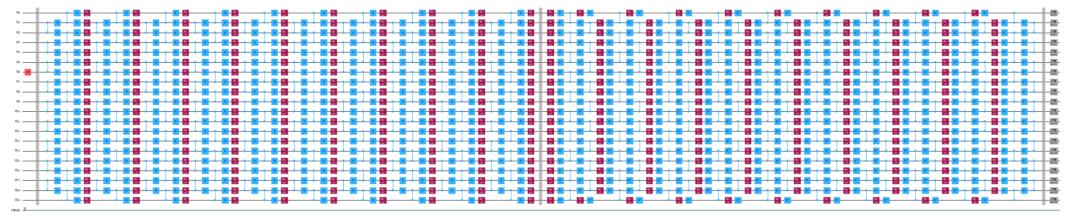
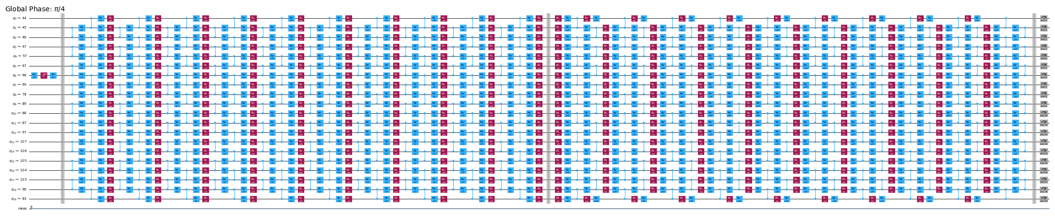
데모의 편의를 위해 1D 미러 이징 체인(mirror Ising chain)을 선택합니다. 1D 이징 체인은 회로 구조가 조밀하여 PEC 구현을 보여주기에 적합합니다. 미러 회로는 예상 결과를 쉽게 알 수 있게 해줍니다(즉, 관측량으로 1을 측정해야 합니다).
또한 미러 회로를 실행하고자 하므로, 회로 후반부의 모든 게이트에 대해 전반부에 역 게이트가 있어야 합니다. 측정 관측량 ****에는 비Z 기저 측정이 포함되어 있으며, Executor가 회로 끝에서 원하는 기저를 처리하므로, 미러 회로의 시작 부분에 적절한 게이트를 삽입하는 prepare_basis 함수를 제공합니다. 이 세부 사항은 미러 회로 데모에 특화된 것입니다. get_measurement_bases 함수를 사용하면 어떤 게이트가 필요하고 어디에 추가해야 하는지 쉽게 파악할 수 있으며, "Prepare canonical bases measurements" 섹션에서 설명하는 box 어노테이션의 관례에서 발생하는 큐비트 인덱스의 미묘한 차이도 추적할 수 있습니다.
num_qubits = 20
target_obs_sparse = [("XZ", [6, 13], 1.0)]
observable = SparsePauliOp.from_sparse_list(target_obs_sparse, num_qubits=num_qubits)
bases_virt, reverser_virt = get_measurement_bases(observable)
num_trotter_steps = 10
rx_angle = np.pi / 4
def construct_ising_circuit(
    num_qubits: int, num_trotter_steps: int, rx_angle: float, barrier: bool = True
) -> QuantumCircuit:
    circuit = QuantumCircuit(num_qubits)

    for _step in range(num_trotter_steps):
        circuit.rx(rx_angle, range(num_qubits))
        if barrier:
            circuit.barrier()
        for first_qubit in (1, 2):
            for idx in range(first_qubit, num_qubits, 2):
                # equivalent to Rzz(-pi/2):
                circuit.sdg([idx - 1, idx])
                circuit.cz(idx - 1, idx)
        if barrier:
            circuit.barrier()

    return circuit

def prepare_basis(circuit: QuantumCircuit, basis: list[int]) -> QuantumCircuit:
    # basis is a list of integer values from 0 to 3. These map to the basis measurement as:
    # 0 = I; 1 = Z; 2 = X; 3 = Y
    assert len(basis) == circuit.num_qubits

    out_circ = circuit.copy_empty_like()
    for qb, bas in enumerate(basis):
        if bas in {0, 1}:
            continue
        if bas == 2:
            out_circ.h(qb)
        elif bas == 3:
            out_circ.rx(-np.pi / 2, qb)

    out_circ.barrier()
    out_circ.compose(circuit, inplace=True)
    return out_circ

def mirror_circuit(circuit: QuantumCircuit, *, inverse_first: bool = False) -> QuantumCircuit:
    mirror_circ = circuit.copy_empty_like()
    mirror_circ.compose(circuit.inverse() if inverse_first else circuit, inplace=True)
    mirror_circ.barrier()
    mirror_circ.compose(circuit if inverse_first else circuit.inverse(), inplace=True)
    mirror_circ.measure_active()
    return mirror_circ
# Instantiate circuit
circuit = construct_ising_circuit(num_qubits, num_trotter_steps, rx_angle, barrier=False)
mirrored_circuit = mirror_circuit(circuit, inverse_first=True)
mirrored_circuit = prepare_basis(mirrored_circuit, bases_virt[0])
mirrored_circuit.draw("mpl", fold=-1, scale=0.3, idle_wires=False, measure_arrows=False)
2단계. 최적화
실행할 회로, 측정할 관측량, 노이즈 학습 파라미터와 관련된 세부 사항을 최적화합니다. 시작점으로, 분수 게이트(fractional gates) 옵션이 활성화된 백엔드를 인스턴스화합니다. 이 분수 게이트는 일부 후선택(post-selection) 필터링에서 더 높은 감도를 제공합니다.
token = "<YOUR_TOKEN>"
instance = "<YOUR_INSTANCE>"

# This is used to retrieve shared results
shared_service = QiskitRuntimeService(
    channel="ibm_quantum_platform",
    token=token,
    instance=instance,
)

# This is used to run on real hardware
service = service = QiskitRuntimeService()
qiskit_runtime_service._discover_account:WARNING:2025-11-10 11:19:40,108: Loading account with the given token. A saved account will not be used.
backend = service.backend("ibm_kingston", use_fractional_gates=True)
먼저, QPU에서 실행하는 데 필요한 ISA 명령어로 회로를 트랜스파일합니다. 이 실험에서 수집된 데이터의 경우, 가장 품질이 높은 체인을 평가하여 큐비트를 수동으로 선택합니다.
layout = [44, 45, 46, 47, 57, 67, 68, 69, 78, 89, 88, 87, 97, 107, 106, 105, 104, 103, 96, 83]
isa_pm = generate_preset_pass_manager(backend=backend, initial_layout=layout, optimization_level=0)

isa_circuit = isa_pm.run(mirrored_circuit)
assert isa_circuit.layout.final_index_layout() == layout

isa_observable = observable.apply_layout(layout, num_qubits=isa_circuit.num_qubits)
2025-11-10 11:19:57,810 INFO base_tasks Pass: ContainsInstruction - 0.00715 (ms)
2025-11-10 11:19:57,811 INFO base_tasks Pass: UnitarySynthesis - 0.00525 (ms)
2025-11-10 11:19:57,811 INFO base_tasks Pass: HighLevelSynthesis - 0.02599 (ms)
2025-11-10 11:19:57,811 INFO base_tasks Pass: BasisTranslator - 0.09131 (ms)
2025-11-10 11:19:57,811 INFO base_tasks Pass: SetLayout - 0.02623 (ms)
2025-11-10 11:19:57,812 INFO base_tasks Pass: FullAncillaAllocation - 0.14400 (ms)
2025-11-10 11:19:57,812 INFO base_tasks Pass: EnlargeWithAncilla - 0.06318 (ms)
2025-11-10 11:19:57,813 INFO base_tasks Pass: ApplyLayout - 0.29802 (ms)
2025-11-10 11:19:57,813 INFO base_tasks Pass: CheckMap - 0.07820 (ms)
2025-11-10 11:19:57,814 INFO base_tasks Pass: FilterOpNodes - 0.33283 (ms)
2025-11-10 11:19:57,814 INFO base_tasks Pass: UnitarySynthesis - 0.00691 (ms)
2025-11-10 11:19:57,814 INFO base_tasks Pass: HighLevelSynthesis - 0.13208 (ms)
2025-11-10 11:19:57,816 INFO base_tasks Pass: BasisTranslator - 1.00303 (ms)
2025-11-10 11:19:57,818 INFO base_tasks Pass: FoldRzzAngle - 1.78719 (ms)
2025-11-10 11:19:57,818 INFO base_tasks Pass: ContainsInstruction - 0.00691 (ms)
2025-11-10 11:19:57,818 INFO base_tasks Pass: InstructionDurationCheck - 0.00405 (ms)
wire_order = layout + [q for q in range(isa_circuit.num_qubits) if q not in layout]
isa_circuit.draw(
    "mpl", fold=-1, scale=0.3, idle_wires=False, wire_order=wire_order, measure_arrows=False
)
회로 박스화(Box the circuit)
구현의 편의를 위해 generate_boxing_pass_manager 트랜스파일 패스를 활용합니다. 이 패스는 회로 명령어를 어노테이션이 달린 박스(box)에 배치합니다. 이 박스들은 PEC의 경우 회로의 어느 위치에 안티노이즈(antinoise)를 주입해야 하는지를 명확히 나타냅니다. 설정에 대한 자세한 내용은 Samplomatic 문서를 참조하세요.
SLC 워크플로우에서는 이후 inject_noise_strategy="individual_modification" 사용이 필요합니다. 이는 회로 내의 각 BoxOp를 고유하게 식별할 수 있게 해주기 때문입니다.
find_unique_box_instructions 함수는 제공된 박스화된 회로를 순회하면서 노이즈 학습 및 노이즈 주입 목적으로 고유한 2Q 레이어 또는 측정값을 가진 것들을 식별합니다.
# Box circuit with Twirl and InjectNoise annotations
boxes_pm = generate_boxing_pass_manager(
    twirling_strategy="active",
    inject_noise_strategy="individual_modification",
    inject_noise_targets="gates",
    measure_annotations="all",
)

boxed_circuit = boxes_pm.run(isa_circuit)

# Find the unique instructions (layers) from boxed circuit
unique_2q_instructions = find_unique_box_instructions(
    boxed_circuit, normalize_annotations=None, undress_boxes=True
)
2025-11-10 11:20:01,088 INFO base_tasks Pass: RemoveBarriers - 0.02289 (ms)
2025-11-10 11:20:01,100 INFO base_tasks Pass: GroupGatesIntoBoxes - 12.38990 (ms)
2025-11-10 11:20:01,101 INFO base_tasks Pass: GroupMeasIntoBoxes - 0.47898 (ms)
2025-11-10 11:20:01,104 INFO base_tasks Pass: AddTerminalRightDressedBoxes - 2.88177 (ms)
2025-11-10 11:20:01,111 INFO base_tasks Pass: AddInjectNoise - 6.66904 (ms)
boxed_circuit.draw(
    "mpl", fold=-1, scale=0.3, idle_wires=False, wire_order=wire_order, measure_arrows=False
)

정규 기저 측정 준비(Prepare canonical bases measurements)
고유한 2Q 레이어를 식별할 때 큐비트의 레이블이 지정되는 방식으로 인해, 큐비트 순서를 추적하는 데 특별한 주의가 필요합니다. 아래에서는 회로 박스화 및 고유 명령어 탐색 시 큐비트 순서가 캡처되는 방식의 결과로, Executor에 제공할 때 큐비트 순서를 적절히 업데이트하는 수단으로 canonical_qubits 개념을 도입합니다. 자세한 내용은 큐비트 순서 규칙 문서를 참조하세요.
# Determine the canonical qubits order
meas_box = boxed_circuit.data[-1]
canonical_qubits = [
    idx for idx, qubit in enumerate(boxed_circuit.qubits) if qubit in meas_box.qubits
]

# map canonical qubit to physical (isa) qubit
c_2_p = {c: p for c, p in enumerate(canonical_qubits)}
# map physical (isa) qubit to virtual qubit (index in original circuit)
p_2_v = {p: v for v, p in enumerate(layout)}
# compute map between virtual and canonical qubit indices.
c_2_v = {c: p_2_v[p] for c, p in c_2_p.items()}

assert len(c_2_v) == num_qubits

bases_canon = [
    np.array([base_i[c_2_v[c]] for c in range(num_qubits)], dtype=np.uint8) for base_i in bases_virt
]
라이트콘 음영, 노이즈 학습, 안티노이즈 주입을 위한 워크플로우
참고: 이 튜토리얼에서 SLC-PEC 구현을 위해, 노이즈 학습이 완료되기 전에 SLC 경계 계산을 실행해서, 완화 대상 회로가 학습된 노이즈 모델과 가능한 한 근접한 시간에 실행되도록 해요. 원칙적으로 이 워크플로우는 동시 실행이 가능하도록 더욱 개선할 수 있어요. 즉, 노이즈 경계를 추정하는 동안 노이즈 학습 작업을 병렬로 실행해요. 임의의 양자 회로의 경우, 노이즈 경계 계산은 약한 지수적 의존성을 가지고 확장될 수 있어요. 따라서 워크플로우의 효율성을 극대화하려면 병렬 실행을 사용하는 것이 바람직할 수 있어요. 이를 위해, 클러스터 기반(128스레드) 리소스를 포함하고 동일한 계산 시간 제한 하에서 랩톱(8스레드)과 비교했을 때 제공된 회로에 대해 더 정교한 경계 집합을 얻을 수 있는 방법을 간략히 시연해요. 또한, 이 워크플로우에서는 구현하지 않았지만, 가장 효율적인 워크플로우를 달성하기 위해 노이즈 학습 및 노이즈 경계 계산을 위한 QPU 실행을 병렬화할 수 있어요.
학습될 노이즈 모델 Pauli 항 예측
generate_noise_model_paulis 함수는 제공된 회로의 각 박스 레이어를 순회하며 회로의 큐비트 연결성을 고려하여 관련된 모든 weight-1 및 weight-2 Pauli 항을 생성하고, 활성 노드와 엣지에 관련된 항을 선택합니다. 이러한 항들은 이후 순방향 및 역방향 노이즈 경계를 계산하는 데 사용됩니다.
noise_model_paulis = generate_noise_model_paulis(
    unique_2q_instructions, backend.coupling_map, boxed_circuit
)
noise_model_rates = {ref: None for ref in noise_model_paulis}
a. 순방향 경계 계산 및 강화
compute_forward_bounds 함수는 각 레이어의 게이트와 위에서 생성된 Pauli 항 사이의 교환 관계를, 순방향 전파 오류가 원하는 관측량 에 미치는 영향 측면에서 평가해요. Pauli 항과 교환 가능한 게이트의 경우 아무 작업도 수행하지 않아요. Clifford 게이트의 경우, 회로의 시작 쪽으로 밀어내요. 비-Clifford 게이트의 경우, 목표 관측량에 대한 영향을 근사해 두고, 이후(모든 경계를 병합한 뒤) 노이즈 소거의 우선순위를 정할 때 사용해요. 이 경계는 먼저 L2 노름(즉, 관련 Pauli 항 계수의 제곱합의 제곱근)을 적용해 얻어요. 관련된 큐비트 항이 너무 많을 경우, 삼각 부등식을 사용하는 더 느슨한 경계로 되돌아가요.
랩톱 수준의 리소스
slc_atol = 1e-8
slc_eigval_max_qubits = 18
slc_evolution_max_terms = 1000
slc_num_processes = 8
slc_timeout = 60
forward_bounds = compute_forward_bounds(
    boxed_circuit,
    noise_model_paulis,
    isa_observable,
    evolution_max_terms=slc_evolution_max_terms,
    eigval_max_qubits=slc_eigval_max_qubits,
    atol=slc_atol,
    num_processes=slc_num_processes,
    timeout=slc_timeout,
)
2025-11-10 11:20:04,344 INFO forward Evolving Pauli error terms forwards through the circuit.
2025-11-10 11:20:04,344 INFO forward Modelling errors as though they happen *after* each noise layer.
2025-11-10 11:20:04,345 INFO remove_measure Removing ANY Measure operations from the provided circuit!
2025-11-10 11:20:04,453 INFO circuit_iter Noisy box 'm39'
2025-11-10 11:20:05,254 INFO circuit_iter Noisy box 'm38'
2025-11-10 11:20:05,304 INFO circuit_iter Noisy box 'm37'
2025-11-10 11:20:05,382 INFO circuit_iter Noisy box 'm36'
2025-11-10 11:20:05,467 INFO circuit_iter Noisy box 'm35'
2025-11-10 11:20:05,580 INFO circuit_iter Noisy box 'm34'
2025-11-10 11:20:05,705 INFO circuit_iter Noisy box 'm33'
2025-11-10 11:20:05,857 INFO circuit_iter Noisy box 'm32'
2025-11-10 11:20:06,034 INFO circuit_iter Noisy box 'm31'
2025-11-10 11:20:06,221 INFO circuit_iter Noisy box 'm30'
2025-11-10 11:20:06,449 INFO circuit_iter Noisy box 'm29'
2025-11-10 11:20:06,724 INFO circuit_iter Noisy box 'm28'
2025-11-10 11:20:07,628 INFO circuit_iter Noisy box 'm27'
2025-11-10 11:20:09,110 INFO circuit_iter Noisy box 'm26'
2025-11-10 11:20:11,696 INFO circuit_iter Noisy box 'm25'
2025-11-10 11:20:16,100 INFO circuit_iter Noisy box 'm24'
2025-11-10 11:20:21,781 INFO circuit_iter Noisy box 'm23'
2025-11-10 11:20:30,244 INFO circuit_iter Noisy box 'm22'
2025-11-10 11:20:40,416 INFO circuit_iter Noisy box 'm21'
2025-11-10 11:20:53,437 INFO circuit_iter Noisy box 'm20'
2025-11-10 11:21:06,038 INFO circuit_iter Noisy box 'm19'
2025-11-10 11:21:06,038 WARNING commutator_bounds Bounds computation timed out.
2025-11-10 11:21:06,039 INFO circuit_iter Noisy box 'm18'
2025-11-10 11:21:06,039 INFO circuit_iter Noisy box 'm17'
2025-11-10 11:21:06,039 INFO circuit_iter Noisy box 'm16'
2025-11-10 11:21:06,040 INFO circuit_iter Noisy box 'm15'
2025-11-10 11:21:06,040 INFO circuit_iter Noisy box 'm14'
2025-11-10 11:21:06,040 INFO circuit_iter Noisy box 'm13'
2025-11-10 11:21:06,040 INFO circuit_iter Noisy box 'm12'
2025-11-10 11:21:06,041 INFO circuit_iter Noisy box 'm11'
2025-11-10 11:21:06,041 INFO circuit_iter Noisy box 'm10'
2025-11-10 11:21:06,041 INFO circuit_iter Noisy box 'm9'
2025-11-10 11:21:06,042 INFO circuit_iter Noisy box 'm8'
2025-11-10 11:21:06,042 INFO circuit_iter Noisy box 'm7'
2025-11-10 11:21:06,042 INFO circuit_iter Noisy box 'm6'
2025-11-10 11:21:06,042 INFO circuit_iter Noisy box 'm5'
2025-11-10 11:21:06,043 INFO circuit_iter Noisy box 'm4'
2025-11-10 11:21:06,043 INFO circuit_iter Noisy box 'm3'
2025-11-10 11:21:06,043 INFO circuit_iter Noisy box 'm2'
2025-11-10 11:21:06,043 INFO circuit_iter Noisy box 'm1'
2025-11-10 11:21:06,044 INFO circuit_iter Noisy box 'm0'
수동 검사를 위한 SLC 시각화
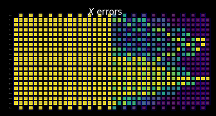
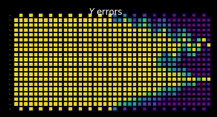
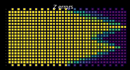
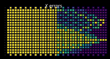
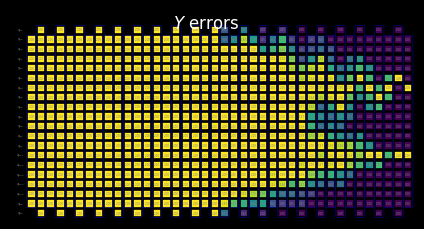
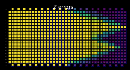
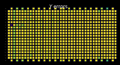
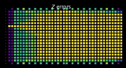
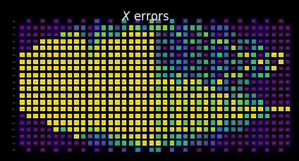
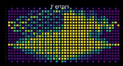
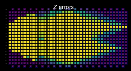
음영 처리된 경계의 동작은 측정값과 Pauli 항이 로컬 오류와 어떻게 상호 작용하는지를 살펴봄으로써 해석할 수 있습니다. 이러한 패턴은 이 kicked Ising Hamiltonian 시간 진화 문제의 특징이며, 논문 Lightcone Shading for Classically Accelerated Quantum Error Mitigation에도 등장하며, 몇 가지 뚜렷한 특징을 가지고 있습니다:
-
관측량의 두 비항등 Pauli에서 발생하는 두 개의 원뿔을 명확히 구분할 수 있습니다.
-
큐비트 6의 X 측정이 가장 오른쪽 레이어의 X 오류와 교환 가능하다는 것을 알 수 있습니다.
-
큐비트 13의 Z Pauli가 가장 오른쪽 레이어의 Z 오류와 교환 가능하다는 것을 알 수 있습니다.
-
위에서 지정한 타임아웃에 도달하면, 왼쪽의 나머지 레이어는 모두 값이 2인 trivial 경계로 채워집니다.
for p in "XYZ":
    display(
        draw_shaded_lightcone(
            boxed_circuit,
            forward_bounds,
            noise_model_paulis,
            pauli_filter=p,
            scale=0.15,
            fold=-1,
            idle_wires=False,
            wire_order=wire_order,
            measure_arrows=False,
        )
    )
b. 순방향 경계 계산 및 조임
다음으로 tighten_with_speed_limit 함수를 사용해 경계를 강화해요. 이 함수는 관측량이 회로를 역방향으로 어떻게 퍼져나가는지를 추적하고, 그 퍼짐을 이용해 각 노이즈 연산자의 영향에 대한 상한을 설정해요. 이때 앞서 계산한 순방향 경계와 역방향 전파 경계 중 더 작은 값을 취해요.
forward_bounds_tighter = tighten_with_speed_limit(
    forward_bounds, boxed_circuit, noise_model_paulis, isa_observable
)
2025-11-10 11:21:08,270 INFO speed_limit Tighting bounds using information propagation speed limits
2025-11-10 11:21:08,270 INFO speed_limit Modelling errors as though they happen *after* each noise layer.
2025-11-10 11:21:08,298 INFO remove_measure Removing ANY Measure operations from the provided circuit!
2025-11-10 11:21:08,310 INFO circuit_iter Noisy box 'm39'
2025-11-10 11:21:08,314 INFO circuit_iter Noisy box 'm38'
2025-11-10 11:21:08,317 INFO circuit_iter Noisy box 'm37'
2025-11-10 11:21:08,319 INFO circuit_iter Noisy box 'm36'
2025-11-10 11:21:08,323 INFO circuit_iter Noisy box 'm35'
2025-11-10 11:21:08,325 INFO circuit_iter Noisy box 'm34'
2025-11-10 11:21:08,328 INFO circuit_iter Noisy box 'm33'
2025-11-10 11:21:08,330 INFO circuit_iter Noisy box 'm32'
2025-11-10 11:21:08,334 INFO circuit_iter Noisy box 'm31'
2025-11-10 11:21:08,336 INFO circuit_iter Noisy box 'm30'
2025-11-10 11:21:08,338 INFO circuit_iter Noisy box 'm29'
2025-11-10 11:21:08,340 INFO circuit_iter Noisy box 'm28'
2025-11-10 11:21:08,344 INFO circuit_iter Noisy box 'm27'
2025-11-10 11:21:08,346 INFO circuit_iter Noisy box 'm26'
2025-11-10 11:21:08,349 INFO circuit_iter Noisy box 'm25'
2025-11-10 11:21:08,351 INFO circuit_iter Noisy box 'm24'
2025-11-10 11:21:08,355 INFO circuit_iter Noisy box 'm23'
2025-11-10 11:21:08,357 INFO circuit_iter Noisy box 'm22'
2025-11-10 11:21:08,360 INFO circuit_iter Noisy box 'm21'
2025-11-10 11:21:08,362 INFO circuit_iter Noisy box 'm20'
2025-11-10 11:21:08,367 INFO circuit_iter Noisy box 'm19'
2025-11-10 11:21:08,369 INFO circuit_iter Noisy box 'm18'
2025-11-10 11:21:08,372 INFO circuit_iter Noisy box 'm17'
2025-11-10 11:21:08,375 INFO circuit_iter Noisy box 'm16'
2025-11-10 11:21:08,378 INFO circuit_iter Noisy box 'm15'
2025-11-10 11:21:08,380 INFO circuit_iter Noisy box 'm14'
2025-11-10 11:21:08,383 INFO circuit_iter Noisy box 'm13'
2025-11-10 11:21:08,386 INFO circuit_iter Noisy box 'm12'
2025-11-10 11:21:08,389 INFO circuit_iter Noisy box 'm11'
2025-11-10 11:21:08,391 INFO circuit_iter Noisy box 'm10'
2025-11-10 11:21:08,394 INFO circuit_iter Noisy box 'm9'
2025-11-10 11:21:08,396 INFO circuit_iter Noisy box 'm8'
2025-11-10 11:21:08,399 INFO circuit_iter Noisy box 'm7'
2025-11-10 11:21:08,401 INFO circuit_iter Noisy box 'm6'
2025-11-10 11:21:08,404 INFO circuit_iter Noisy box 'm5'
2025-11-10 11:21:08,406 INFO circuit_iter Noisy box 'm4'
2025-11-10 11:21:08,410 INFO circuit_iter Noisy box 'm3'
2025-11-10 11:21:08,412 INFO circuit_iter Noisy box 'm2'
2025-11-10 11:21:08,415 INFO circuit_iter Noisy box 'm1'
2025-11-10 11:21:08,417 INFO circuit_iter Noisy box 'm0'
수동 검사를 위한 SLC 시각화
라이트콘 제한을 고려하여 경계를 더욱 조일 수 있습니다. 원칙적으로, 이를 통해 계산된 경계에서 타임아웃 이후에 설정된 trivial 경계로의 전환이 더 부드러워집니다. 여기서는 라이트콘이 이미 회로의 끝에 도달했기 때문에 그 효과가 뚜렷하게 나타나지 않습니다.
for p in "XYZ":
    display(
        draw_shaded_lightcone(
            boxed_circuit,
            forward_bounds_tighter,
            noise_model_paulis,
            pauli_filter=p,
            scale=0.15,
            fold=-1,
            idle_wires=False,
            wire_order=wire_order,
            measure_arrows=False,
        )
    )
c. 역방향 경계 계산
노이즈 예측의 이 부분은 특정 레이어에서의 오류가 입력 상태 에 어떤 영향을 미칠 수 있는지를 평가합니다. compute_backward_bounds 함수는 먼저 회로를 반전시키고 측정 게이트를 제거한 다음, 순방향 경계 계산에서 수행된 것과 유사한 분석을 진행합니다.
backward_bounds = compute_backward_bounds(
    boxed_circuit,
    noise_model_paulis,
    evolution_max_terms=slc_evolution_max_terms,
    num_processes=slc_num_processes,
    timeout=slc_timeout,
)
2025-11-10 11:21:10,666 INFO backward Evolving Pauli error terms backwards through the circuit.
2025-11-10 11:21:10,666 INFO backward Modelling errors as though they happen *after* each noise layer.
2025-11-10 11:21:10,667 INFO remove_measure Removing ANY Measure operations from the provided circuit!
2025-11-10 11:21:10,774 INFO circuit_iter Noisy box 'm0'
2025-11-10 11:21:11,640 INFO circuit_iter Noisy box 'm1'
2025-11-10 11:21:11,681 INFO circuit_iter Noisy box 'm2'
2025-11-10 11:21:11,867 INFO circuit_iter Noisy box 'm3'
2025-11-10 11:21:12,078 INFO circuit_iter Noisy box 'm4'
2025-11-10 11:21:12,329 INFO circuit_iter Noisy box 'm5'
2025-11-10 11:21:12,637 INFO circuit_iter Noisy box 'm6'
2025-11-10 11:21:13,110 INFO circuit_iter Noisy box 'm7'
2025-11-10 11:21:13,705 INFO circuit_iter Noisy box 'm8'
2025-11-10 11:21:14,384 INFO circuit_iter Noisy box 'm9'
2025-11-10 11:21:15,213 INFO circuit_iter Noisy box 'm10'
2025-11-10 11:21:15,946 INFO circuit_iter Noisy box 'm11'
2025-11-10 11:21:16,754 INFO circuit_iter Noisy box 'm12'
2025-11-10 11:21:17,557 INFO circuit_iter Noisy box 'm13'
2025-11-10 11:21:18,447 INFO circuit_iter Noisy box 'm14'
2025-11-10 11:21:19,453 INFO circuit_iter Noisy box 'm15'
2025-11-10 11:21:20,472 INFO circuit_iter Noisy box 'm16'
2025-11-10 11:21:21,479 INFO circuit_iter Noisy box 'm17'
2025-11-10 11:21:22,660 INFO circuit_iter Noisy box 'm18'
2025-11-10 11:21:23,705 INFO circuit_iter Noisy box 'm19'
2025-11-10 11:21:24,849 INFO circuit_iter Noisy box 'm20'
2025-11-10 11:21:26,030 INFO circuit_iter Noisy box 'm21'
2025-11-10 11:21:27,111 INFO circuit_iter Noisy box 'm22'
2025-11-10 11:21:28,354 INFO circuit_iter Noisy box 'm23'
2025-11-10 11:21:29,554 INFO circuit_iter Noisy box 'm24'
2025-11-10 11:21:30,897 INFO circuit_iter Noisy box 'm25'
2025-11-10 11:21:32,113 INFO circuit_iter Noisy box 'm26'
2025-11-10 11:21:33,622 INFO circuit_iter Noisy box 'm27'
2025-11-10 11:21:34,962 INFO circuit_iter Noisy box 'm28'
2025-11-10 11:21:36,504 INFO circuit_iter Noisy box 'm29'
2025-11-10 11:21:38,021 INFO circuit_iter Noisy box 'm30'
2025-11-10 11:21:39,750 INFO circuit_iter Noisy box 'm31'
2025-11-10 11:21:41,237 INFO circuit_iter Noisy box 'm32'
2025-11-10 11:21:42,974 INFO circuit_iter Noisy box 'm33'
2025-11-10 11:21:44,527 INFO circuit_iter Noisy box 'm34'
2025-11-10 11:21:46,535 INFO circuit_iter Noisy box 'm35'
2025-11-10 11:21:48,152 INFO circuit_iter Noisy box 'm36'
2025-11-10 11:21:50,074 INFO circuit_iter Noisy box 'm37'
2025-11-10 11:21:51,814 INFO circuit_iter Noisy box 'm38'
2025-11-10 11:21:53,943 INFO circuit_iter Noisy box 'm39'
수동 검사를 위한 SLC 시각화
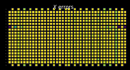
역방향 경계를 계산하면서, 초기 상태의 구조가 오류 전파의 초기 동작을 어떻게 지배하는지 확인할 수 있습니다:
-
Z 오류가 초기에 |0⟩ 초기 상태와 어떻게 교환(commute)되는지 명확하게 볼 수 있습니다.
-
X 기저의 +1 고유 상태로 초기화되는 큐비트 6에서만 Z 오류가 교환에 실패하며, X 오류는 교환됩니다.
for p in "XYZ":
    display(
        draw_shaded_lightcone(
            boxed_circuit,
            backward_bounds,
            noise_model_paulis,
            pauli_filter=p,
            scale=0.15,
            fold=-1,
            idle_wires=False,
            wire_order=wire_order,
            measure_arrows=False,
        )
    )
학습된 노이즈 율 없이 병합된 경계 미리보기
merged_bounds 함수는 원하는 관측량에 대한 총 추정 편향을 최소화하기 위해 역방향 경계에서 순방향 경계로 전환하는 회로 내 지점을 결정합니다. 이 편향은 해당 지점 이전의 모든 노이즈 위치에 대한 역방향 경계 기여분과 그 이후의 모든 노이즈 위치에 대한 순방향 경계 기여분의 합으로 계산됩니다. 현재 이는 모든 큐비트에 대해 균일하게 수행됩니다.
중요 참고 사항: 순방향 경계에서 역방향 경계로 전환하는 지점은 학습된 노이즈 율에 따라 달라집니다.
merged_bounds = merge_bounds(
    boxed_circuit,
    forward_bounds_tighter,
    backward_bounds,
    noise_model_rates,
)
2025-11-10 11:21:58,304 WARNING merge Missing noise rates. Partitioning backward/forward commutator bounds by assuming uniform error rates.
2025-11-10 11:21:58,305 WARNING merge Optimal spacetime partitioning not implemented!Just partitioning list of noisy boxes.
2025-11-10 11:21:58,305 INFO merge Determined Box idx for partitioning to be 20.
수동 검사를 위한 SLC 시각화
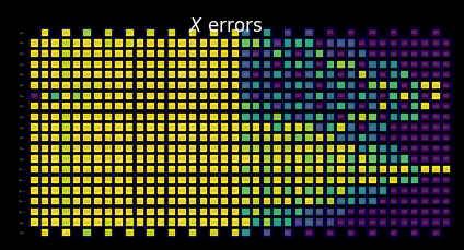
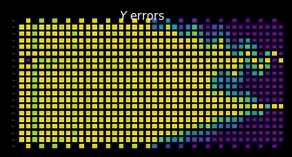
역방향 경계와 조여진 순방향 경계를 병합한 후, 결합된 SLC의 동작이 명확해집니다:
-
위의 함수는 역방향 경계에서 조여진 순방향 경계로 전환되는 파티션이 선택됨을 알려줍니다.
-
아래에서 SLC가 이제 부분적인 역방향 경계와 부분적인 조여진 순방향 경계를 포함하고 있음을 확인할 수 있습니다.
for p in "XYZ":
    display(
        draw_shaded_lightcone(
            boxed_circuit,
            merged_bounds,
            noise_model_paulis,
            pauli_filter=p,
            scale=0.15,
            fold=-1,
            idle_wires=False,
            wire_order=wire_order,
            measure_arrows=False,
        )
    )
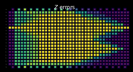
클러스터 수준 리소스
여기서는 클러스터의 128개 스레드를 활용하면 랩톱과 동일한 계산 시간 내에서도 이 더 큰 회로의 상당 부분을 전파할 수 있음을 보여줘요.
with open("exp_data/merged_bounds_cluster.pickle", "rb") as file:
    merged_bounds_cluster = pickle.load(file)
for p in "XYZ":
    display(
        draw_shaded_lightcone(
            boxed_circuit,
            merged_bounds_cluster,
            noise_model_paulis,
            pauli_filter=p,
            scale=0.15,
            fold=-1,
            idle_wires=False,
            wire_order=wire_order,
            measure_arrows=False,
        )
    )
3단계. 실행
이 섹션에서는 실제 양자 디바이스를 사용하는 워크플로우 단계를 시작합니다. 이 학습 기반 오류 완화 방법에는 두 가지 단계가 있습니다:
-
NoiseLeanerV3를 사용해 노이즈를 학습해요. -
새로운 Samplomatic 및 Estimator 프레임워크를 사용해 오류 완화 회로를 실행해요.
양자 회로에서 얻은 경계 오류를 바탕으로, 오류 예산을 우선순위화하고, 샘플링 오버헤드를 결정하며, QPU에서 실행하기 위해 관련 노이즈 율을 학습해야 합니다. 또한 이 노이즈 율 정보를 통해 클러스터의 강력한 컴퓨팅 자원을 활용하여 동일한 잔류 편향을 유지하면서 샘플링 오버헤드를 줄이는 방법을 강조할 수 있습니다.
a. 노이즈율 학습
노이즈 학습기는 Probabilistic error cancellation with sparse Pauli-Lindblad models on noisy quantum processors 논문에 설명된 Pauli-Lindblad 노이즈 모델을 기반으로, 관심 있는 하나 이상의 회로에 영향을 미치는 노이즈 프로세스를 특성화할 수 있게 해줍니다. run() 메서드는 노이즈 학습기 구성에 지정된 옵션을 기반으로 제공된 고유한 2-큐비트 레이어에 대한 노이즈 학습 작업을 시작합니다. 이 옵션에서 Pauli-twirling 전략을 조정할 수 있으며, 이는 하드웨어가 Pauli-Lindblad 노이즈 모델에 의해 잘 설명되도록 보장하는 데 도움이 됩니다.
노이즈 모델의 세부 사항은 시간이 지남에 따라 변동될 위험이 있습니다. 따라서 4시간이 지난 실험에 대해 학습된 노이즈 모델이 재계산되도록 매개변수를 설정합니다. 이는 대략적인 경험칙이므로 자신의 작업에 적용할 때는 신중하게 고려해야 합니다.
post_selection_enabled = True
load_cached_noise_results = True
noise_learner_options = NoiseLearnerV3Options(
    num_randomizations=64,
    shots_per_randomization=128,
    layer_pair_depths=[1, 2, 4, 8, 12, 16, 24, 32, 40, 48],
    post_selection={
        "enable": post_selection_enabled,
        "strategy": "edge",
        "x_pulse_type": "rx",
    },
)

noise_learner = NoiseLearnerV3(backend, noise_learner_options)
if load_cached_noise_results:
    noise_learner_job = shared_service.job("d46ssf71gh7s7398k9a0")
else:
    noise_learner_job = noise_learner.run(unique_2q_instructions)
noise_learner_result = noise_learner_job.result()
if post_selection_enabled:
    print("Minimum fraction of shots kept for noise learning experiments: ", end="")
    print(
        f"{min([min(d.values()) for d in [nlr.metadata['post_selection']['fraction_kept'] for nlr in noise_learner_result[:2]]]):.2f}"
    )
Minimum fraction of shots kept for noise learning experiments: 0.58
# Get a dict mapping InjectNoise.ref to QubitSparsePaulilist
refs_2_plm = noise_learner_result.to_dict(unique_2q_instructions, require_refs=False)
b.i. 실제로 학습한 노이즈율로 병합된 경계 업데이트
이제 특정 노이즈 모델이 학습되었으므로, 학습된 노이즈 율을 예측된 노이즈 경계에 적용하고 편향 최소화에 가장 큰 영향을 미치는 경계를 최종적으로 결정할 수 있습니다.
merged_bounds = merge_bounds(
    boxed_circuit,
    forward_bounds_tighter,
    backward_bounds,
    refs_2_plm,
)
2025-11-10 11:22:03,755 WARNING merge Optimal spacetime partitioning not implemented!Just partitioning list of noisy boxes.
2025-11-10 11:22:03,756 INFO merge Determined Box idx for partitioning to be 20.
b.ii. 하드웨어 실행을 위한 local_scales 계산
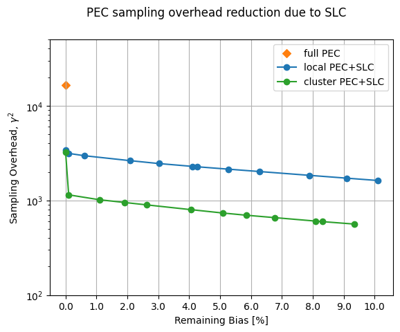
compute_local_scales는 회로 내의 각 가능한 노이즈 오류를 살펴보고, 해당 오류가 최종 측정 결과를 얼마나 편향시킬 수 있는지, 그리고 이를 수정하는 데 얼마나 비용이 드는지를 추정합니다. 그런 다음 가치 대비 효율을 기준으로 오류의 순위를 매기고, 허용된 샘플링 비용 예산 내에서 (또는 원하는 정확도를 달성하면서) 편향을 최대한 줄이는 부분 집합을 선택합니다. 결과는 어떤 오류를 적극적으로 완화하고 어떤 오류를 완화하지 않을지를 나타내는 스케일링 인수 집합(local_scales)과 함께, 예측된 총 샘플링 비용 오버헤드(sampling_costs) 및 잔류 편향(residual_bias_bound)을 제공합니다.
원하는 잔류 편향을 제어하는 능력은 PEC의 SLC 구현에서 중요한 기능입니다. 원래 구현에서는 샘플링 오버헤드가 항상 편향 제로를 목표로 했지만, 예상 잔류 편향과의 트레이드오프를 통해 필요한 샘플링 오버헤드를 조정할 수 있습니다. 이를 통해 사용자는 고정된 샘플링 예산 내에 머물 수 있으며, 워크플로우를 처음 프로토타입화할 때 특히 유용합니다.
id_map = map_modifier_ref_to_ref(boxed_circuit)
summed_rates = 0.0
for _box_id, noise_id in id_map.items():
    learned_plm = refs_2_plm[noise_id]
    summed_rates += np.sum(learned_plm.rates)
    # print(f"{_box_id}:\tgamma = {np.exp(2 * summed_rates):1.6e}\tsampling cost = {np.exp(4 * summed_rates):1.6e}")
total_gamma = np.exp(2 * summed_rates)
print(f"Full PEC gamma={total_gamma}, sampling cost (gamma^2) = {total_gamma**2}")
Full PEC gamma=128.56055005423153, sampling cost (gamma^2) = 16527.81503024657
biases = []
costs = []
for bias in [0.0, *np.arange(0.001, 0.102, 0.01).tolist()]:
    _, cost_, bias_ = compute_local_scales(
        boxed_circuit,
        merged_bounds,
        refs_2_plm,
        sampling_cost_budget=np.inf,
        bias_tolerance=bias,
    )
    biases.append(bias_)
    costs.append(cost_)
biases_cluster = []
costs_cluster = []
for bias in [0.0, *np.arange(0.001, 0.102, 0.01).tolist()]:
    _, cost_, bias_ = compute_local_scales(
        boxed_circuit,
        merged_bounds_cluster,
        refs_2_plm,
        sampling_cost_budget=np.inf,
        bias_tolerance=bias,
    )
    biases_cluster.append(bias_)
    costs_cluster.append(cost_)
주어진 고전 계산 시간에 대한 샘플링 오버헤드 감소를 위한 클러스터의 이점
xticks = np.arange(0, 11)

fig, ax = plt.subplots()
ax.scatter([0], [total_gamma**2], marker="D", c="tab:orange", label="full PEC")
ax.plot(100 * np.array(biases), np.array(costs), "o-", c="tab:blue", label="local PEC+SLC")
ax.plot(
    100 * np.array(biases_cluster),
    np.array(costs_cluster),
    "o-",
    c="tab:green",
    label="cluster PEC+SLC",
)
ax.set_yscale("log")
ax.set_ylim([100, 50000])
ax.set_xticks(xticks, [f"{x:.1f}" for x in xticks])

ax.set_xlabel("Remaining Bias [%]")
ax.set_ylabel(r"Sampling Overhead, $\gamma^2$")
ax.grid()
ax.legend()
fig.suptitle("PEC sampling overhead reduction due to SLC")
Text(0.5, 0.98, 'PEC sampling overhead reduction due to SLC')
chosen_bias_thres = 0.1
local_scales, sampling_cost, residual_bias_bound = compute_local_scales(
    boxed_circuit,
    merged_bounds_cluster,
    refs_2_plm,
    sampling_cost_budget=np.inf,
    bias_tolerance=chosen_bias_thres,
)
print(
    f"PEC+SLC sampling cost (gamma^2) = {sampling_cost} w/ remaining bias = {100 * residual_bias_bound:.1f}%"
)
PEC+SLC sampling cost (gamma^2) = 563.1803982530477 w/ remaining bias = 9.3%
c. 안티노이즈를 사용해 관심 회로 실행
c.i. samplex를 사용해 템플릿 회로 준비
samplex는 Samplomatic의 build 메서드의 출력으로, template_circuit에 대한 무작위 파라미터를 생성하는 데 필요한 모든 정보를 인코딩합니다. 이는 QuantumProgram 객체를 설정하는 데 사용되며, 이 객체들은 Executor 프리미티브를 통해 QPU에서 실행됩니다. 각 QuantumProgram은 여러 항목을 포함할 수 있으며, 이를 template과 samplex의 쌍으로 생각할 수 있습니다.
자세한 내용은 Hello samplomatic 튜토리얼을 참조하세요.
# Build template circuit and samplex for later use with the "Executor"
template_circuit, samplex = samplomatic.build(boxed_circuit)
# Set up postselection if it's been enabled
if post_selection_enabled:
    # Set up post selection PM (to add PS instructions)
    post_selection_pm = PassManager(
        [
            AddSpectatorMeasures(backend.coupling_map),
            AddPostSelectionMeasures(x_pulse_type="rx"),
        ]
    )
    final_template_circuit = post_selection_pm.run(template_circuit)
else:
    final_template_circuit = template_circuit
2025-11-10 11:22:04,839 INFO base_tasks Pass: AddSpectatorMeasures - 3.41392 (ms)
2025-11-10 11:22:04,843 INFO base_tasks Pass: AddPostSelectionMeasures - 2.88510 (ms)
c.ii. QuantumProgram 설정
num_randomizations = 4096
shots_per_randomization = 64
chunk_size = 256
# Set up QuantumProgram
program = QuantumProgram(shots=shots_per_randomization, noise_maps=refs_2_plm)

# no EM

# Collect up a dict of the other arguments that need to be bound to samplex_inputs
samplex_inputs = {f"noise_scales.{ref}": float(0) for ref in local_scales}
samplex_inputs |= {"basis_changes": {"basis0": bases_canon[0]}}

# Convert samplex_inputs into a dict to pass to QuantumProgram
samplex_arguments = samplex.inputs().bind(**samplex_inputs).make_broadcastable()

program.append(
    circuit=final_template_circuit,
    samplex=samplex,
    samplex_arguments=samplex_arguments,
    shape=(num_randomizations,),
    chunk_size=chunk_size,
)

# plain PEC

# Collect a dict of the other arguments that need to be bound to samplex_inputs
samplex_inputs = {f"noise_scales.{ref}": float(-1) for ref in local_scales}
samplex_inputs |= {"basis_changes": {"basis0": bases_canon[0]}}

# Convert samplex_inputs into a dict to pass to QuantumProgram
samplex_arguments = samplex.inputs().bind(**samplex_inputs).make_broadcastable()

program.append(
    circuit=final_template_circuit,
    samplex=samplex,
    samplex_arguments=samplex_arguments,
    shape=(num_randomizations,),
    chunk_size=chunk_size,
)

# PEC+SLC

# Collect a dict of the other arguments that need to be bound to samplex_inputs
samplex_inputs = {f"noise_scales.{ref}": float(-1) for ref in local_scales}
samplex_inputs |= {"basis_changes": {"basis0": bases_canon[0]}}
samplex_inputs |= {"local_scales": local_scales}

# Convert samplex_inputs into a dict to pass to QuantumProgram
samplex_arguments = samplex.inputs().bind(**samplex_inputs).make_broadcastable()

program.append(
    circuit=final_template_circuit,
    samplex=samplex,
    samplex_arguments=samplex_arguments,
    shape=(num_randomizations,),
    chunk_size=chunk_size,
)
c.iii. Executor 프리미티브로 프로그램 실행
executor = Executor(backend)
load_cached_executor_results = True
if load_cached_executor_results:
    job_exec = shared_service.job("d46t1q6qsa9s73cb28g0")
else:
    job_exec = executor.run(program)
results_exec = job_exec.result()
Step 4. 후처리(Post-process)
expectation_values를 사용해 최종 기댓값을 계산할 때, 가능한 한 최고 품질의 결과를 얻을 수 있도록 몇 가지 유용한 후처리 기법을 구현해요. 먼저, 판독(readout) 과정에서 발생하는 오류를 처리하는 트위르드 판독 완화(TREX)를 적용해요. 그런 다음, Heron 백엔드에서 비-마르코프(non-Markovian) 노이즈로 인한 오류를 후선택(post-selection) 방법을 통해 수정해요. 이 방법은 활성 큐비트와 스펙테이터(spectator) 큐비트를 측정한 후, 각 큐비트에 느린 회전을 적용하고, 다시 한번 측정해요. 두 측정값이 예상대로 뒤집힌 큐비트를 확인하지 못하는 경우, PostSelector 함수의 mask를 적용해 해당 샷을 버려요. 마스크 계산 내에서, 단일 큐비트 노드 또는 인접한 스펙테이터 에지를 기준으로 필터링하는 특정 전략을 설정할 수 있으며, 이는 필터링되는 샷의 수와 결과의 품질 모두에 영향을 미칠 수 있어요.
measurement_noise_map = noise_learner_result[2].to_pauli_lindblad_map()
trex_scale_factors = trex_factors(measurement_noise_map, reverser_virt)
post_selection_strategy = "node"
def post_process_conv(datum, steps=16, gamma=None, ps=False, trex=False):
    meas = datum["meas"]
    flips = datum["measurement_flips.meas"]
    signs = datum.get("pauli_signs", None)

    meas_basis_axis = None
    avg_axis = 0

    mask = None
    if ps and post_selection_enabled:
        # Post-select the results
        post_selector = PostSelector.from_circuit(
            circuit=final_template_circuit, coupling_map=backend.coupling_map
        )

        # Compute the ps mask for filtering results
        mask = post_selector.compute_mask(datum, strategy=post_selection_strategy)

        # Compute fraction of shots kept from post selection
        total_num_shots = num_randomizations * shots_per_randomization
        ps_ratio = np.sum(mask) * 100 / total_num_shots / len(bases_canon)
        print(
            f"With {post_selection_strategy}-based post selection ({ps_ratio:.1f}% of shots kept):"
        )

    results = []
    for i in range(steps, num_randomizations + 1, steps):
        # Compute mitigated expvals w/out postselectoion
        res = executor_expectation_values(
            meas[:i],
            reverser_virt,
            meas_basis_axis,
            avg_axis=avg_axis,
            measurement_flips=flips[:i],
            pauli_signs=signs[:i] if signs is not None else None,
            postselect_mask=mask[:i] if mask is not None else None,
            rescale_factors=trex_scale_factors if trex else None,
            gamma_factor=gamma,
        )
        results.append(res[0])
    return results
gamma_pec = gamma_from_noisy_boxes(refs_2_plm, id_map)
gamma_slc = gamma_from_noisy_boxes(refs_2_plm, id_map, local_scales)
steps = 16
results = {}

for label, result_idx, gamma, use_ps, use_trex in [
    ("PEC", 1, gamma_pec, True, True),
    ("PEC+SLC", 2, gamma_slc, True, True),
    ("Unmitigated", 0, None, False, False),
]:
    res = post_process_conv(
        results_exec[result_idx], steps=steps, gamma=gamma, ps=use_ps, trex=use_trex
    )
    results[label] = res
With node-based post selection (27.0% of shots kept):
With node-based post selection (26.8% of shots kept):
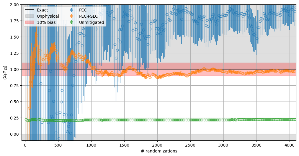
실험 결과를 살펴보면, PEC, SLC와 결합된 PEC, 그리고 완화되지 않은(unmitigated) 결과라는 기본값(baseline), 이렇게 서로 다른 접근 방식의 동작을 직접 비교할 수 있습니다. 강조할 몇 가지 구체적인 사항은 다음과 같습니다:
-
완화되지 않은 결과는 원하는 편향(bias) 범위를 벗어난 상태로 남아 있으며, 샘플링 오버헤드의 영향을 받지 않습니다.
-
위에서 계산된 높은 샘플링 비용(~10k)을 고려할 때, PEC 단독으로는 사용된 랜덤화 한도 내에서 수렴하지 않습니다.
-
반면에 PEC + SLC는 훨씬 빠르게 수렴합니다.
-
또한 오차 범위도 일반 PEC보다 PEC + SLC에서 훨씬 빠르게 감소합니다.
fig, ax = plt.subplots(1, 1, figsize=(12, 6))

ax.axhline(1.0, color="black", label="Exact")
ax.fill_between([-50, 4100], -10, 0, color="grey", alpha=0.25, label="Unphysical")
ax.fill_between([-50, 4100], 1, 10, color="grey", alpha=0.25)
ax.fill_between([-50, 4100], 0.9, 1.1, color="red", alpha=0.25, label="10% bias")

for label, res in results.items():
    ax.errorbar(
        list(range(steps, num_randomizations + 1, steps)),
        [r[0] for r in res],
        yerr=[r[1] for r in res],
        alpha=0.75,
        marker="o",
        linestyle="",
        markerfacecolor="none",
        label=label,
    )

ax.set_ylabel(r"$\langle X_{6}Z_{13}\rangle$")
ax.set_xlabel("# randomizations")
ax.grid()

ax.legend(ncols=2)
ax.set_ylim([-0.1, 2.0])
ax.set_xlim([-50, 4100])
(-50.0, 4100.0)