시공간 코드를 이용한 저오버헤드 오류 검출

사용량 추정치: Heron 프로세서(ibm_kingston 또는 이에 준하는 프로세서) 기준 4분 (참고: 이는 추정치일 뿐입니다. 실제 실행 시간은 다를 수 있습니다.)

학습 목표

• 시공간 파울리 검사가 클리포드 회로에서 논리적 오류를 어떻게 검출하는지, 그리고 검사 신드롬에 대한 사후 선택이 샘플링된 분포의 충실도를 어떻게 높이는지.

• get_check_qubits, NoiseModel, add_pauli_checks를 사용하여 qiskit-paulice 패키지로 하드웨어 효율적인 검사를 자동으로 찾아 삽입하는 방법.

• 안정자 상태의 안정자를 샘플링하고 검사 신드롬에 대해 사후 선택함으로써 안정자 상태의 충실도를 추정하는 방법.

• IBM Quantum® 하드웨어에서 전체 오류 검출 워크플로를 실행하고 노이즈가 있는 충실도와 사후 선택된 충실도를 비교하는 방법.

전제 조건

• 유틸리티 규모 양자 컴퓨팅을 위한 하드웨어 기초.

• 클리포드 및 안정자 형식체계, 그리고 안정자 그룹이 순수 안정자 상태를 어떻게 기술하는지.

배경

Simon Martiel과 Ali Javadi-Abhari가 작성한 시공간 코드를 이용한 저오버헤드 오류 검출 [1]은 완전한 오류 정정과 더 가벼운 오류 완화 사이에 위치하는, 클리포드가 주를 이루는 회로에서 논리적 오류를 검출하는 방법을 소개합니다. 이 아이디어는 van den Berg 등이 작성한 일관 파울리 검사를 통한 단발성 오류 완화 [2]의 일관 파울리 검사(CPC)를 기반으로 합니다. 두 접근법 모두, 클리포드 "페이로드" 회로가 특정 불변량을 확인하기 위해 보조 큐비트와 얽히게 됩니다. 보조 큐비트를 측정하면 실행 중 오류가 검출되었는지를 알려주는 신드롬이 생성됩니다. 검출된 오류가 없는 샘플만 유지하면 사후 선택률이 낮아지는 대가로 샘플링된 분포의 충실도가 향상됩니다.

일관 파울리 검사와 시공간 검사의 핵심 차이는 측정하는 연산자에 있습니다. 일관 파울리 검사는 시간적으로 국소화된 고가중치 연산자를 측정합니다. 헤비헥스와 같이 연결성이 제한된 큐비트 토폴로지에서는 이러한 검사에 많은 SWAP 게이트가 필요하며, 이로 인해 회로가 실제로 실행하기에는 너무 깊어지는 경우가 많습니다. 대신 검사를 시공간 코드로 구현하면 각 검사가 페이로드 회로 전체에 공간적, 시간적으로 분산됩니다. 이는 큐비트 및 깊이 오버헤드를 낮게 유지하면서도 논리적 오류 검출에 효과적인 하드웨어 효율적 인코딩을 만들어냅니다.

qiskit-paulice 패키지가 하는 일

qiskit-paulice 패키지는 이러한 검사의 구축을 자동화하여 직접 손으로 만들 필요가 없게 해줍니다. 이 패키지의 주된 역할은 오류 검출을 극대화하면서 큐비트 오버헤드를 최소화하는 회로 내 위치에 유효한 시공간 파울리 검사를 찾아 삽입하는 것입니다. 검사는 그 연산자가 페이로드 회로의 논리적 동작을 변경하지 않을 때 유효하고, 얽힘 게이트를 적게 사용할 때 저가중치이며, 검사 자체가 도입하는 노이즈에 비해 상당 부분의 오류를 검출할 때 효과적입니다. 이 패키지는 노이즈 모델에 대해 후보 검사들을 점수화하고 가장 좋은 것들을 회로에 반영합니다. 이 튜토리얼에서는 세 가지 API 메서드를 사용합니다.

• get_check_qubits는 백엔드 커플링 맵을 검사하고 목표 및 보조 큐비트 쌍을 반환합니다. target_qubits[i]에 대한 검사는 ancilla_qubits[i]를 사용합니다.

• NoiseModel.from_backend는 백엔드 벤치마크 데이터로부터 대략적인 노이즈 모델을 구축합니다. 이 모델은 후보 검사를 점수화하는 데 사용되므로, 정확하게 학습된 노이즈 모델이 필요하지는 않습니다. 학습된 파울리-린드블라드 모델에 대해서는 NoiseModel.from_pauli_lindblad_maps를 참고하세요.

• add_pauli_checks는 회로에서 검사를 찾아 삽입합니다. 이 함수는 검사 개수가 점점 늘어나는 CheckedCircuit 객체의 시퀀스를 반환하며, 각 객체는 측정된 비트스트링을 신드롬 벡터로 매핑하는 get_postselection_method를 제공합니다. cost 인수는 검사를 점수화하는 함수를 선택합니다(gamma, 사후 선택된 역노이즈 채널의 샘플링 오버헤드, 또는 LER, 논리적 오류율). method 인수는 탐색 전략을 선택합니다(windowed, genetic, 또는 windowed_genetic). 이 튜토리얼에서는 cost="gamma"와 method="windowed"를 사용하는데, 이는 결정론적이고 재현 가능한 검사 선택을 제공합니다.

안정자 샘플링을 통한 충실도 추정

오류 검출이 얼마나 잘 작동하는지 측정하기 위해, 회로가 이상적으로 준비하는 안정자 상태 $|\psi\rangle = U|0\rangle^{\otimes n}$의 충실도를 하드웨어가 실제로 출력하는 노이즈가 있는 상태 $\rho$에 대해 추정할 수 있습니다. 순수 안정자 상태 $|\psi\rangle$에 대한 사영 연산자는 안정자 그룹 $\mathcal{S}$의 $2^n$개 원소에 대한 균일 평균과 같습니다.

$|\psi\rangle\langle\psi| = \frac{1}{2^n}\sum_{G \in \mathcal{S}} G.$

이를 충실도 식에 대입하면, $\rho$의 충실도는 $\rho$에 대한 모든 안정자 $G \in \mathcal{S}$의 기댓값의 평균으로 주어집니다.

$F = \mathrm{Tr}(\rho|\psi\rangle\langle\psi|) = \frac{1}{2^n} \sum_{G \in \mathcal{S}} \mathrm{Tr}(\rho G) = \frac{1}{2^n} \sum_{G \in \mathcal{S}} \langle G \rangle_\rho.$

더 큰 문제의 경우 $2^n$개의 모든 안정자를 열거하는 것이 불가능하므로, 무작위 표본으로부터 충실도를 추정할 수 있습니다. $\mathcal{S}$에서 균일하게 무작위로 $M$개의 안정자 $G_1, \ldots, G_M$을 뽑으면 비편향 추정량을 얻습니다.

$\hat F_M = \frac{1}{M} \sum_{i=1}^M \langle G_i \rangle_\rho.$

클리포드 회로는 안정자 상태를 준비하므로, 안정자들의 샘플링된 기댓값으로부터 그 충실도를 직접 추정할 수 있습니다. 이 튜토리얼은 먼저 작은 회로로 시뮬레이터에서 워크플로를 살펴본 다음, 더 크고 깊은 회로로 하드웨어에서 동일한 워크플로를 실행합니다. 회로에 비-클리포드 연산이 많이 포함될수록 유효한 검사의 수가 빠르게 줄어들기 때문에, 이 방법은 클리포드가 주를 이루는 회로에서 가장 잘 작동합니다.

요구 사항

이 튜토리얼을 시작하기 전에 다음 사항이 설치되어 있는지 확인하세요.

• 시각화 지원이 포함된 Qiskit SDK v2.0 이상

• Qiskit Runtime v0.40 이상 (pip install qiskit-ibm-runtime)

• Qiskit Aer v0.17 이상 (pip install qiskit-aer)

• Qiskit Paulice (pip install qiskit-paulice)

• tqdm (pip install tqdm)

설정

필요한 라이브러리를 가져오고, 임포트로 제공되지 않는 헬퍼 함수를 정의합니다. random_clifford_circuit 함수는 벽돌쌓기(brickwork) 무작위 클리포드 페이로드를 구축하고, find_check_layout은 백엔드 커플링 맵에서 사용 가능한 보조 큐비트가 많은 저오류 큐비트 경로를 탐색하며, learned_noise_model은 NoiseLearner의 출력을 qiskit-paulice 노이즈 모델로 변환하고, append_basis_rotation은 안정자가 계산 기저에서 측정되도록 회로를 회전시키며, expectation은 샘플링된 카운트로부터 안정자 기댓값을 계산하고, cum_mean_sem은 진행 중인 충실도 추정치를 추적합니다.

# Added by doQumentation — required packages for this notebook
!pip install -q matplotlib numpy qiskit qiskit-aer qiskit-ibm-runtime qiskit-paulice tqdm

# Standard library imports
import random
import time

# External libraries
import matplotlib.pyplot as plt
import numpy as np
from tqdm import tqdm

# Qiskit
from qiskit import QuantumCircuit
from qiskit.quantum_info import Clifford, Pauli, PauliLindbladMap, PauliList
from qiskit.result import sampled_expectation_value
from qiskit.transpiler import generate_preset_pass_manager
from qiskit.visualization import plot_coupling_map

# Qiskit Aer
from qiskit_aer import AerSimulator
from qiskit_aer.noise import NoiseModel as AerNoiseModel
from qiskit_aer.noise import ReadoutError, depolarizing_error

# Qiskit IBM Runtime
from qiskit_ibm_runtime import NoiseLearner, QiskitRuntimeService
from qiskit_ibm_runtime import SamplerV2 as Sampler

# Qiskit Paulice
from qiskit_paulice import add_pauli_checks
from qiskit_paulice.layout import get_check_qubits
from qiskit_paulice.noise_models import NoiseModel

def random_clifford_circuit(
    num_qubits: int, depth: int, rng: np.random.Generator
) -> QuantumCircuit:
    """Brickwork random Clifford on `num_qubits`, with `depth` CZ layers."""
    qc = QuantumCircuit(num_qubits)
    qc.h(range(num_qubits))
    for d in range(depth):
        for i in range(d % 2, num_qubits - 1, 2):
            qc.cz(i, i + 1)
        for q in range(num_qubits):
            if rng.integers(0, 2):
                qc.sx(q)
            if rng.integers(0, 2):
                qc.s(q)
            if rng.integers(0, 2):
                qc.sx(q)
    return qc

def find_check_layout(
    backend,
    num_qubits: int,
    rng: np.random.Generator,
    num_trials: int = 200,
    max_gate_error: float = 0.03,
    max_readout_error: float = 0.2,
) -> list[int]:
    """Find a low-error path of `num_qubits` qubits with many available ancillas.

    Builds random self-avoiding walks on the coupling map, excluding the qubits
    and two-qubit gates whose reported errors exceed the thresholds, and keeps
    the path that offers the most target and ancilla pairs. Ties are broken by
    the lower average two-qubit gate error along the path.
    """
    target = backend.target
    gate_2q = next(
        name for name in ("cz", "ecr", "cx") if name in target.operation_names
    )

    # Collect per-edge gate errors and per-qubit readout errors
    edge_error = {}
    for qubits, props in target[gate_2q].items():
        edge = tuple(sorted(qubits))
        if props is not None and props.error is not None:
            edge_error[edge] = min(edge_error.get(edge, 1.0), props.error)
    readout_error = {
        qubit: target["measure"][(qubit,)].error
        for (qubit,) in target["measure"]
    }

    # Keep only the edges whose gate and readout errors are acceptable
    adjacency = {}
    for (q1, q2), error in edge_error.items():
        if (
            error <= max_gate_error
            and readout_error.get(q1, 1.0) <= max_readout_error
            and readout_error.get(q2, 1.0) <= max_readout_error
        ):
            adjacency.setdefault(q1, set()).add(q2)
            adjacency.setdefault(q2, set()).add(q1)

    # Random self-avoiding walks; keep the path with the most check pairs
    starts = sorted(adjacency)
    best_path = None
    best_score = (-1, float("inf"))
    for _ in range(num_trials):
        path = [starts[rng.integers(len(starts))]]
        while len(path) < num_qubits:
            options = sorted(adjacency[path[-1]] - set(path))
            if not options:
                break
            path.append(options[rng.integers(len(options))])
        if len(path) < num_qubits:
            continue
        num_pairs = len(get_check_qubits(backend.coupling_map, path)[0])
        mean_error = float(
            np.mean(
                [edge_error[tuple(sorted(e))] for e in zip(path, path[1:])]
            )
        )
        if num_pairs > best_score[0] or (
            num_pairs == best_score[0] and mean_error < best_score[1]
        ):
            best_path, best_score = path, (num_pairs, mean_error)

    if best_path is None:
        raise RuntimeError(
            "No connected low-error path found. Relax the error thresholds."
        )
    return best_path

def learned_noise_model(layer_errors, layout: list[int]) -> NoiseModel:
    """Build a `NoiseModel` from `NoiseLearner` results.

    `NoiseLearner` reports one `PauliLindbladError` per entangling layer, whose
    generators are indexed against that layer's own physical qubits, while
    `NoiseModel.from_pauli_lindblad_maps` expects `PauliLindbladMap`s indexed the
    way `NoiseModel.from_backend` indexes them: by position in `layout`. This
    translates between the two and drops generators that fall outside `layout`.
    """
    phys_to_virt = {phys: virt for virt, phys in enumerate(layout)}
    maps = []
    for layer in layer_errors:
        if layer.error is None:
            continue
        terms = []
        for pauli, rate in zip(
            layer.error.generators, layer.error.rates, strict=True
        ):
            label, indices = [], []
            for local, phys in enumerate(layer.qubits):
                x, z = bool(pauli.x[local]), bool(pauli.z[local])
                if not (x or z):
                    continue
                if phys not in phys_to_virt:
                    break  # generator reaches outside the layout, so skip it
                label.append("Y" if x and z else "X" if x else "Z")
                indices.append(phys_to_virt[phys])
            else:
                if label:
                    terms.append(
                        ("".join(label), tuple(indices), float(rate))
                    )
        # Each map needs a 2-qubit generator to define an entangling layer
        if any(len(t[1]) == 2 for t in terms):
            maps.append(
                PauliLindbladMap.from_sparse_list(
                    terms, num_qubits=len(layout)
                )
            )
    if not maps:
        raise RuntimeError(
            "No usable layer errors. Check that the learner ran on this layout."
        )
    return NoiseModel.from_pauli_lindblad_maps(maps)

def append_basis_rotation(
    circuit: QuantumCircuit, pauli: Pauli
) -> QuantumCircuit:
    """Strip measurements, append basis rotations for `pauli`, and re-measure."""
    out = circuit.remove_final_measurements(inplace=False)
    for q in range(pauli.num_qubits):
        if pauli.x[q]:
            if pauli.z[q]:
                out.sdg(q)
            out.h(q)
    out.measure_all()
    return out

def expectation(counts: dict, pauli: Pauli) -> float:
    """Expectation value of `pauli` from counts measured in the Z basis.

    Pads with identity on any qubits beyond the support of `pauli`, such as the
    check ancillas that appear in the postselected counts.
    """
    if not counts:
        return float("nan")
    n = pauli.num_qubits
    sign = -1 if int(pauli.phase) % 4 == 2 else 1
    total = len(next(iter(counts)))
    label = "".join(
        "Z" if q < n and (pauli.x[q] or pauli.z[q]) else "I"
        for q in range(total - 1, -1, -1)
    )
    return sign * sampled_expectation_value(counts, label)

def cum_mean_sem(values: np.ndarray):
    """Cumulative mean and standard error of the mean, ignoring NaNs."""
    valid = ~np.isnan(values)
    total = np.cumsum(np.where(valid, values, 0.0))
    total_sq = np.cumsum(np.where(valid, values**2, 0.0))
    count = np.maximum(np.cumsum(valid).astype(float), 1)
    mean = total / count
    sem = np.sqrt(np.maximum(total_sq / count - mean**2, 0) / count)
    return np.where(np.cumsum(valid) > 0, mean, np.nan), sem

소규모 시뮬레이터 예제

이 섹션에서는 노이즈가 있는 시뮬레이터에서 전체 워크플로를 살펴봅니다. 백엔드 벤치마크 데이터를 사용하여 큐비트 레이아웃과 노이즈 모델을 선택하고, 검사를 자동으로 찾아내며, 샘플링된 분포에 대한 사후 선택을 사용하여 충실도 개선을 보여줍니다.

1단계: 고전적 입력을 양자 문제로 매핑

페이로드 회로는 얕은 1차원 벽돌쌓기 무작위 클리포드 회로입니다. 이 회로는 클리포드이므로, 샘플링된 안정자 기댓값으로부터 직접 충실도를 추정할 수 있는 안정자 상태를 준비합니다. 다음 단계에서 검사를 시각화하기 쉽도록 얕은 회로로 시작합니다.

num_qubits = 12
depth = 4
seed = 1764
rng = np.random.default_rng(seed)
np.random.seed(seed)

circuit = random_clifford_circuit(num_qubits, depth, rng)
circuit.measure_all()
circuit.draw("mpl", fold=-1, scale=0.6)

2단계: 양자 하드웨어 실행을 위한 최적화

회로를 하드웨어에 매핑하면 물리적 큐비트 레이아웃, 후보 검사를 점수화하는 노이즈 모델, 그리고 검사 자체가 설정됩니다.

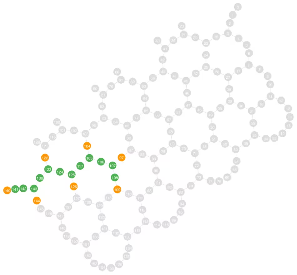
먼저 백엔드를 선택하고, 설정 섹션에서 정의한 find_check_layout 헬퍼를 사용하여 커플링 맵에서 1차원 큐비트 레이아웃을 탐색합니다. 이 헬퍼는 오류율이 가장 높은 게이트와 판독을 피하는 무작위 자기 회피 보행을 구축하고, 가장 많은 목표-보조 쌍을 제공하는 경로를 유지합니다. 탐색이 백엔드 자체로부터 연결성과 오류 데이터를 읽어오기 때문에, 동일한 코드가 어떤 IBM Quantum QPU에서도 실행됩니다. 그런 다음 get_check_qubits 함수가 목표 및 보조 쌍을 반환하며, target_qubits[i]에 대한 검사는 ancilla_qubits[i]를 사용합니다.

다음 커플링 그래프에서 초록색 큐비트는 페이로드 큐비트이고 주황색 큐비트는 검사를 구현하는 보조 큐비트입니다. 인접한 보조 큐비트가 있는 큐비트는 검사의 목표 큐비트로 사용됩니다.

service = QiskitRuntimeService()
backend = service.least_busy(operational=True, simulator=False)

print(f"Backend: {backend.name}")

# Search for a low-error path, then pair each target qubit with a neighboring ancilla
layout = find_check_layout(backend, num_qubits, rng)
target_qubits, ancilla_qubits = get_check_qubits(backend, layout)
num_checks = len(target_qubits)

print(f"Target qubits:  {target_qubits}")
print(f"Ancilla qubits: {ancilla_qubits}")
plot_coupling_map(
    num_qubits=backend.num_qubits,
    qubit_coordinates=getattr(
        backend.configuration(), "qubit_coordinates", None
    ),
    coupling_map=backend.configuration().coupling_map,
    figsize=(12, 12),
    qubit_color=[
        "#4CAF50"
        if i in set(layout)
        else "#FF9800"
        if i in set(ancilla_qubits)
        else "#DDDDDD"
        for i in backend.coupling_map.graph.node_indices()
    ],
    qubit_size=220,
    line_width=2,
    font_size=90,
)

Backend: ibm_boston
Target qubits:  [105, 107, 108, 123, 125, 141, 143]
Ancilla qubits: [104, 97, 109, 122, 126, 140, 144]

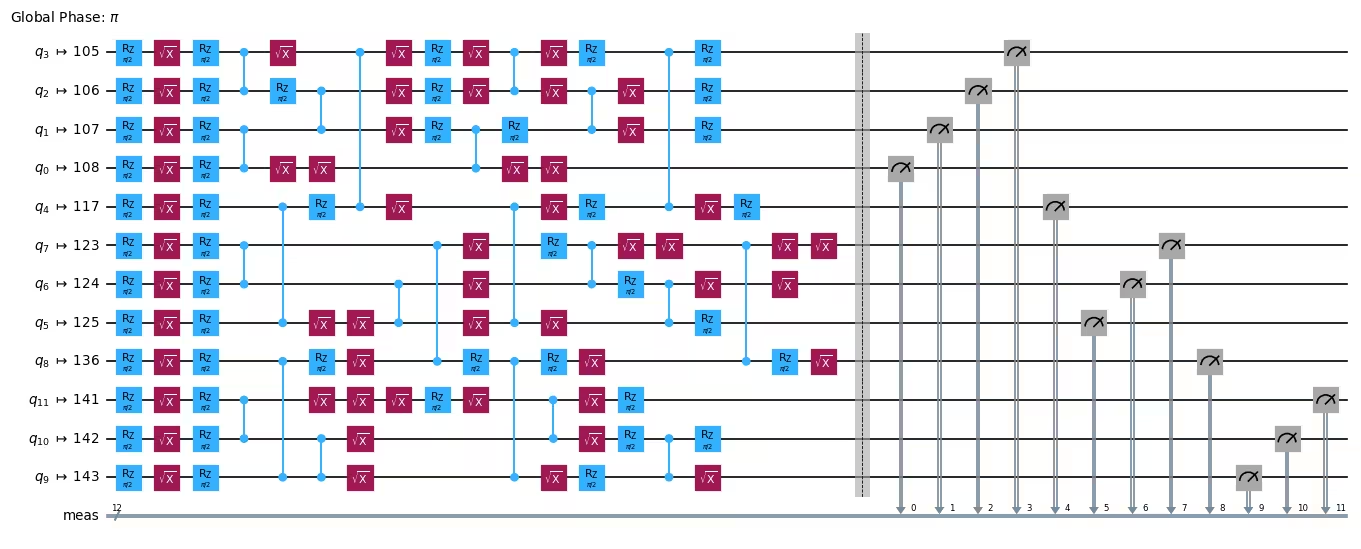
백엔드와 레이아웃이 선택되면, 페이로드를 명령어 집합 아키텍처(ISA) 회로로 트랜스파일합니다. 레이아웃을 설정하고 게이트를 백엔드의 네이티브 게이트 집합으로 변환하기만 하면 됩니다.

pm = generate_preset_pass_manager(
    optimization_level=0, backend=backend, initial_layout=layout
)
circuit_isa = pm.run(circuit)
circuit_isa.draw("mpl", fold=-1, scale=0.6)

다음으로, 백엔드의 게이트 및 판독 노이즈가 실행에 미치는 영향을 모델링합니다. 노이즈 모델은 회로 내에서 검사가 가장 많은 오류를 포착하는 위치를 결정합니다. 더 정확한 모델은 검출 성능을 향상시키지만, 대개 QPU를 샘플링하여 학습할 필요는 없습니다. 다음 모델은 qiskit-ibm-runtime 벤치마크 데이터로부터 게이트 및 판독 노이즈에 대한 균일 감극 채널을 추론합니다.

noise_model = NoiseModel.from_backend(
    backend, layout, uniform_gate_noise=True
)
print(noise_model)

NoiseModel(gate_noise=0.001079865281450939, readout_noise=0.006001790364583333, idling_noise=None)

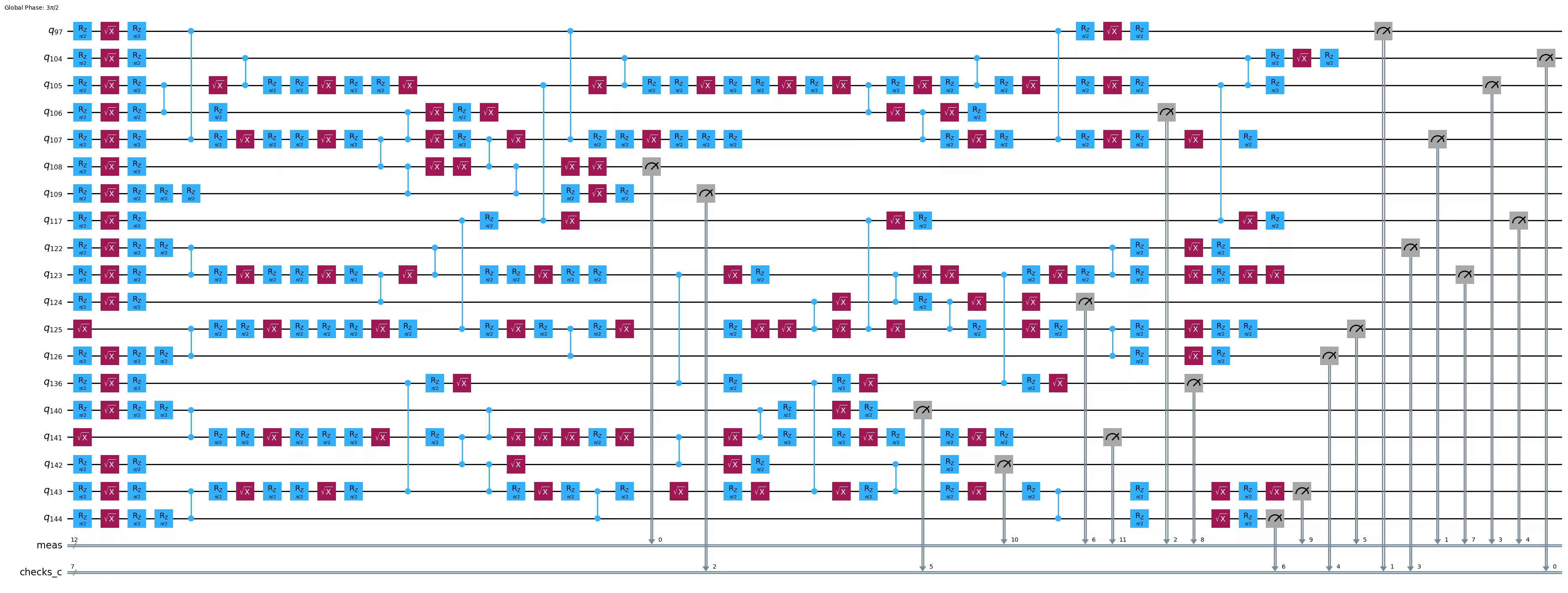
이제 회로에 검사를 추가합니다. add_pauli_checks 함수는 클리포드 페이로드, 목표 큐비트 목록, 노이즈 모델을 입력으로 받습니다. ancilla_qubits 인수는 각 목표와 짝지을 물리적 보조 큐비트를 함수에 알려줍니다. 검사는 목표 큐비트가 나타나는 순서대로 추가되므로, 검사된 회로의 최종 레이아웃은 layout + ancilla_qubits가 됩니다. 검사 개수(i)가 더 적은 출력 회로를 실행하려면 최종 레이아웃은 layout + ancilla_qubits[:i]가 됩니다.

add_pauli_checks의 출력은 검사가 없는 것부터 모든 목표 큐비트에 검사가 하나씩 있는 것까지, 검사 개수가 점점 늘어나는 회로들의 시퀀스입니다. 시각화를 통해 검사가 지정된 목표 및 보조 쌍을 사용함을 확인할 수 있습니다. 좋은 검사를 찾는 방법에 대한 자세한 내용은 참고문헌 [1]의 보충 정보 II절부터 IV절을 참고하세요.

checked = add_pauli_checks(
    circuit_isa,
    target_qubits,
    noise_model,
    ancilla_qubits=ancilla_qubits,
    cost="gamma",
    method="windowed",
    seed=seed,
)

print(f"Physical layout of payload and ancillas: {layout + ancilla_qubits}")
print("Checked circuit:")
checked[-1].circuit.draw("mpl", fold=-1, idle_wires=False)

Physical layout of payload and ancillas: [108, 107, 106, 105, 117, 125, 124, 123, 136, 143, 142, 141, 104, 97, 109, 122, 126, 140, 144]
Checked circuit:

3단계: Qiskit 프리미티브를 사용한 실행

게이트 노이즈의 영향을 눈에 보이게 하기 위해, 페이로드의 깊이를 늘리고 그 안정자들 중 일부를 샘플링합니다. 각 안정자는 일반적으로 다른 안정자들과 큐비트별로 교환되지 않으므로, 단일 검사 집합이 두 개의 서로 다른 안정자 모두에 대해 유효하지는 않습니다. 안정자들을 교환 가능한 집합으로 묶는 대신, 각 안정자에 대해 독립적으로 좋은 검사 집합을 찾습니다. 안정자를 균일하게 무작위로 샘플링하면 비편향 충실도 추정치를 얻습니다.

더 깊은 회로를 구축하고 그 안정자들 중 무작위 표본을 추출합니다.

depth = 24
num_stabilizers = 20
num_shots = 1_000

circuit = random_clifford_circuit(num_qubits, depth, rng)

# Build the full stabilizer group, then sample from it uniformly at random
circ_no_meas = circuit.remove_final_measurements(inplace=False)
stabilizer_group = PauliList([Pauli("I" * num_qubits)])
for generator in (
    Pauli(label) for label in Clifford(circ_no_meas).to_labels(mode="S")
):
    stabilizer_group = stabilizer_group + stabilizer_group.compose(generator)

keep = np.where(
    stabilizer_group.x.any(axis=1) | stabilizer_group.z.any(axis=1)
)[0]
chosen = np.random.default_rng(seed).choice(
    keep, size=min(num_stabilizers, len(keep)), replace=False
)
stabilizers = [stabilizer_group[int(i)] for i in chosen]

two_qubit_depth = circuit.depth(lambda x: x.operation.num_qubits == 2)
print(
    f"Sampled {len(stabilizers)} stabilizers of a {circuit.num_qubits}-qubit "
    f"circuit with two-qubit depth {two_qubit_depth}: "
    f"{{{stabilizers[0]}, {stabilizers[1]}, ...}}"
)

Sampled 20 stabilizers of a 12-qubit circuit with two-qubit depth 24: {ZXIIXZYYXIZZ, XXXYIIZYXIII, ...}

각 샘플링된 안정자에 대해, 안정자가 계산 기저에서 측정되도록 회로를 회전시키고, 이를 백엔드로 트랜스파일한 다음, 좋은 검사 집합을 찾습니다. 각 목표가 자신의 보조 큐비트를 유지하도록 목표와 보조 쌍은 각 안정자마다 함께 섞입니다. 검사는 목표 큐비트가 주어진 순서대로 순차적으로 반영되며, 이미 반영된 검사는 더 많은 검사가 추가되어도 변경되지 않는다는 점을 기억하세요.

noisy_circuits = []
checked_circuits = []
depths_2q = []
t0 = time.time()
for i, pauli in enumerate(tqdm(stabilizers)):
    noisy_circuits.append(pm.run(append_basis_rotation(circuit, pauli)))
    # Shuffle target and ancilla pairs together so each target keeps its ancilla
    targets, ancillas = zip(
        *random.sample(
            list(zip(target_qubits, ancilla_qubits, strict=True)),
            k=len(target_qubits),
        ),
        strict=True,
    )
    checked_circuits.append(
        add_pauli_checks(
            noisy_circuits[-1],
            list(targets),
            noise_model,
            ancilla_qubits=list(ancillas),
            cost="gamma",
            method="windowed",
            seed=seed + 1 + i,
        )
    )
    depths_2q.append(
        checked_circuits[-1][-1].circuit.depth(lambda x: len(x.qubits) == 2)
    )

print(
    f"Added {num_checks} checks to {len(stabilizers)} circuits "
    f"in {(time.time() - t0):.0f}s."
)
print(
    f"On average, two-qubit depth increased from "
    f"{circuit.depth(lambda x: len(x.qubits) == 2)} to {int(np.mean(depths_2q))} "
    f"when adding {num_checks} checks."
)

100%|██████████| 20/20 [00:15<00:00,  1.29it/s]

Added 7 checks to 20 circuits in 15s.
On average, two-qubit depth increased from 24 to 33 when adding 7 checks.

Qiskit Aer로 검사가 없는 페이로드와 검사된 회로들을 샘플링합니다. 시뮬레이터는 검사를 점수화하는 데 사용된 것과 동일한 감극 모델을 사용하므로, 검사가 대상으로 하는 노이즈가 시뮬레이터가 적용하는 노이즈와 같습니다.

aer_nm = AerNoiseModel()
aer_nm.add_all_qubit_quantum_error(
    depolarizing_error(noise_model.gate_noise, 2), ["cz"]
)
p = noise_model.readout_noise
aer_nm.add_all_qubit_readout_error(ReadoutError([[1 - p, p], [p, 1 - p]]))
noisy_sim = AerSimulator(method="stabilizer", noise_model=aer_nm)

counts = []
for i, checked_circ_result in enumerate(tqdm(checked_circuits)):
    noisy_counts = (
        noisy_sim.run(
            noisy_circuits[i], shots=num_shots, seed_simulator=seed * i + 1
        )
        .result()
        .get_counts()
    )
    checked_counts_per_variant = []
    for k, ck in enumerate(checked_circ_result):
        variant_counts = (
            noisy_sim.run(
                ck.circuit, shots=num_shots, seed_simulator=seed * i + 2 + k
            )
            .result()
            .get_counts()
        )
        checked_counts_per_variant.append(variant_counts)
    counts.append((noisy_counts, checked_counts_per_variant))

100%|██████████| 20/20 [00:17<00:00,  1.13it/s]

4단계: 원하는 고전적 형식으로 후처리하고 결과 반환

각 검사는 하나의 보조 큐비트와 하나의 목표 큐비트 사이의 얽힘 게이트를 사용합니다. 보조 큐비트는 $|0\rangle$에서 시작하므로 $Z_\text{anc}$는 그 입력을 안정화합니다. $Z_\text{anc}$를 검사된 회로를 통해 앞으로 전파하면 출력에 대한 파울리 연산자가 생성되며, 그 비항등원 항들이 검사의 서포트를 정의합니다. 검사는 서포트의 비트들이 짝수 패리티를 가질 때 통과합니다. 모든 검사가 통과할 때만 샘플이 유지됩니다.

각 CheckedCircuit의 get_postselection_method는 측정된 비트스트링을 신드롬 벡터로 매핑하는 함수를 반환합니다. 모든 검사에 대해 신드롬이 0인 샘플만 유지하고 나머지는 버립니다. 다음 차트는 검사를 더 추가할수록 사후 선택률이 낮아짐을 보여줍니다. 사후 선택률이 낮을수록 목표 정확도에 도달하기 위해 더 많은 샷이 필요하므로, 검출 능력과 샘플링 비용 사이에는 트레이드오프가 존재합니다. 사후 선택률은 수렴하는 것처럼 보이는데, 이는 추가 검사가 기여하는 검출 능력이 줄어든다는 것을 나타냅니다.

rate_per_variant = []
kept_per_stab = []
for i, (_, checked_counts_per_variant) in enumerate(counts):
    rates = []
    kept_at_num_checks = None
    for k, variant_counts in enumerate(checked_counts_per_variant):
        ps_fn = checked_circuits[i][k].get_postselection_method()
        kept = {
            bs: n for bs, n in variant_counts.items() if not ps_fn(bs).any()
        }
        rates.append(sum(kept.values()) / num_shots)
        if k == num_checks:
            kept_at_num_checks = kept
    rate_per_variant.append(rates)
    kept_per_stab.append(kept_at_num_checks)

max_len = max(len(s) for s in rate_per_variant)
rates_arr = np.full((len(rate_per_variant), max_len), np.nan)
for i, s in enumerate(rate_per_variant):
    rates_arr[i, : len(s)] = s
ks = np.arange(max_len)

fig, ax = plt.subplots(figsize=(8, 4))
ax.plot(ks, rates_arr.T, color="#ff8c00", alpha=0.15, linewidth=1)
ax.plot(
    ks,
    np.nanmedian(rates_arr, axis=0),
    color="black",
    linewidth=1,
    linestyle="--",
    label="median",
)
ax.set_xlabel("Checks committed")
ax.set_ylabel("Postselection rate")
ax.set_ylim((0, 1.05))
ax.set_title(
    f"Per-stabilizer postselection rate ({len(rates_arr)} stabilizers)"
)
ax.legend()
ax.grid(True, alpha=0.3)
plt.tight_layout()
plt.show()

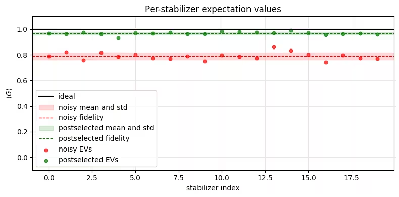
이제 검사가 없는 노이즈 상태의 충실도와 사후 선택된 상태의 충실도를 비교합니다. 검출된 오류가 없는 샘플만 사후 선택하면 모든 안정자의 기댓값이 높아지고, 따라서 추정된 충실도도 높아집니다. 사후 선택된 값은 원시 값보다 적은 샘플을 사용하지만, 기댓값은 더 정확하고 샘플링 분산은 더 낮습니다. 또한 평균 사후 선택률이 노이즈 충실도에 가깝다는 점에 주목하세요. 이는 검사가 거의 모든 오류가 있는 샘플을 검출할 때 예상되는 결과입니다. 모든 검사를 통과하는 샘플의 비율은 오류가 없는 샘플의 비율, 즉 노이즈 상태의 충실도에 가까워집니다.

results = []
for i, ((noisy_counts, _), kept) in enumerate(
    zip(counts, kept_per_stab, strict=True)
):
    results.append(
        (
            expectation(noisy_counts, stabilizers[i]),
            expectation(kept, stabilizers[i]),
            sum(kept.values()) / num_shots,
        )
    )

fidelity_noisy = float(np.nanmean([r[0] for r in results]))
fidelity_postsel = float(np.nanmean([r[1] for r in results]))
psr = float(np.mean([r[2] for r in results]))
print(
    f"ideal fidelity:          1.0\n"
    f"noisy fidelity:          {fidelity_noisy:.4f}\n"
    f"postselected fidelity:   {fidelity_postsel:.4f}\n"
    f"mean postselection rate: {psr:.3f}"
)

evs_ideal = np.ones(len(results))
evs_noisy = np.array([r[0] for r in results])
evs_post = np.array([r[1] for r in results])
idx = np.arange(len(results))

def strip(ax, ys, color, label):
    m, s = np.nanmean(ys), np.nanstd(ys)
    ax.axhspan(
        m - s, m + s, color=color, alpha=0.15, label=f"{label} mean and std"
    )
    ax.axhline(
        m, color=color, linewidth=1, linestyle="--", label=f"{label} fidelity"
    )

fig, ax = plt.subplots(figsize=(8, 4))
ax.axhline(np.nanmean(evs_ideal), color="black", linewidth=1.5, label="ideal")
strip(ax, evs_noisy, "red", "noisy")
strip(ax, evs_post, "green", "postselected")
ax.scatter(idx, evs_noisy, color="red", s=22, alpha=0.7, label="noisy EVs")
ax.scatter(
    idx,
    evs_post,
    color="green",
    s=22,
    alpha=0.7,
    label="postselected EVs",
)
ax.set_xlabel("stabilizer index")
ax.set_ylabel(r"$\langle G \rangle$")
ax.set_ylim((-0.1, 1.1))
ax.set_title("Per-stabilizer expectation values")
ax.legend(loc="lower left")
ax.grid(True, alpha=0.3)
plt.tight_layout()
plt.show()

M = np.arange(1, len(results) + 1)
fig, ax = plt.subplots(figsize=(8, 4))
for ys, color, label in [
    (evs_ideal, "black", "ideal"),
    (evs_noisy, "red", "noisy"),
    (evs_post, "green", "postselected"),
]:
    cm, sem = cum_mean_sem(ys)
    ax.plot(M, cm, color=color, linewidth=1.5, label=label)
    ax.fill_between(M, cm - sem, cm + sem, color=color, alpha=0.15)
ax.set_xlabel("number of stabilizers averaged")
ax.set_ylabel("running fidelity estimate")
ax.set_title("Fidelity convergence versus number of stabilizers")
ax.legend()
ax.grid(True, alpha=0.3)
plt.tight_layout()
plt.show()

ideal fidelity:          1.0
noisy fidelity:          0.7899
postselected fidelity:   0.9679
mean postselection rate: 0.780

감마 점수는 모델링된 노이즈 채널 중 검사가 검출하지 못한 부분이 얼마인지를 나타냅니다. 감마 점수를 반영된 검사 수에 대해 플로팅하면 각 검사가 추가됨에 따라 검출 능력이 어떻게 향상되는지 알 수 있습니다. 값이 1.0이면 검사가 모델링된 노이즈를 모두 포착함을 의미합니다. 더 많은 검사가 반영될수록 곡선은 1.0을 향해 떨어지는데, 이는 추가되는 각 검사가 남아있는 미검출 오류의 일부를 포착함을 보여줍니다.

stab_scores = [
    [variant.cost for variant in checked_circ_result]
    for checked_circ_result in checked_circuits
]
max_len = max(len(s) for s in stab_scores)
scores = np.full((len(stab_scores), max_len), np.nan)
for i, s in enumerate(stab_scores):
    scores[i, : len(s)] = s
ks = np.arange(max_len)

fig, ax = plt.subplots(figsize=(8, 4))
ax.plot(ks, scores.T, color="#4682b4", alpha=0.15, linewidth=1)
ax.plot(
    ks,
    np.nanmedian(scores, axis=0),
    color="black",
    linewidth=1,
    linestyle="--",
    label="median",
)
ax.set_xlabel("Checks committed")
ax.set_ylabel("Gamma")
ax.set_yscale("log")
ax.set_title(f"Per-stabilizer gamma curves ({len(scores)} stabilizers)")
ax.legend()
ax.grid(True, alpha=0.3, which="both")
plt.tight_layout()
plt.show()

대규모 하드웨어 예제

동일한 워크플로가 더 크고 더 깊은 페이로드로 하드웨어에서 실행됩니다. 이 섹션은 시뮬레이터 예제와 동일한 백엔드를 재사용하지만, 자체적인 목표 및 보조 쌍과 패스 매니저를 갖는 새로운 20큐비트 레이아웃을 구축한 다음, 회로들을 하나의 작업으로 QPU에 제출합니다. 이 규모에서는 대부분의 샷이 최소 하나의 검사를 발동시키므로 사후 선택률이 낮으며, 각 회로는 충분한 샘플이 살아남도록 큰 샷 예산이 필요합니다. 따라서 이 예제는 몇 개의 샘플링된 안정자에 예산을 집중합니다. 이는 여전히 비편향 충실도 추정치이지만, 많은 안정자에 대해 평균을 내는 시뮬레이터 예제보다는 더 거친(coarse) 추정치입니다.

시뮬레이터 예제와 비교했을 때 한 가지가 달라집니다. 캘리브레이션 데이터로부터 균일한 감극 채널을 추론하는 대신, 이 섹션에서는 NoiseLearner로 노이즈 모델을 학습하고 그 결과로부터 NoiseModel.from_pauli_lindblad_maps를 사용해 qiskit-paulice 모델을 만듭니다. 학습된 Pauli-Lindblad 모델은 모든 엣지가 동일하게 노이즈가 있다고 가정하는 대신, 이 특정 레이아웃에서의 노이즈의 공간적 구조를 포착하므로, 검사 배치는 QPU에 영향을 미치는 노이즈와 더 유사한 노이즈에 대해 점수가 매겨집니다. 노이즈를 학습하려면 QPU 샘플링이 필요하므로 전체 QPU 샘플링 예산에 반영해야 합니다.

이어지는 매개변수들은 큐비트 수, 깊이, 안정자(stabilizer) 수, 샷 수를 설정합니다. hw_num_shots는 사후 선택(postselection) 비율의 역수에 비례하여 스케일하세요. 3%의 비율에서는 40,000샷이 회로당 약 1,200개의 사후 선택된 샘플을 남깁니다. hw_num_stabilizers를 늘리면 작업당 회로 수가 늘어나는 대가로 더 정밀한 충실도 추정치를 얻을 수 있으며, 각 회로는 동일한 샷 예산이 필요합니다.

단계 1-4 (하나의 코드 블록으로 압축)

다음 셀은 시뮬레이터 예제와 동일한 네 단계를 실행합니다. 더 큰 페이로드를 구성하고 몇 개의 안정자를 샘플링합니다(단계 1). 레이아웃을 선택하고 그 위에서 노이즈 모델을 학습한 다음 각 안정자에 대해 완전히 검사된 회로를 찾습니다(단계 2). 검사가 없는 회로와 검사된 회로를 모두 포함하는 하나의 Sampler 작업을 제출합니다(단계 3). 그리고 검사된 카운트를 사후 선택하여 노이즈가 있는 충실도 추정치와 사후 선택된 충실도 추정치를 안정자별 및 평균으로 비교합니다(단계 4). 이 크기에서는 시뮬레이터 예제처럼 전체 안정자 그룹을 열거하는 것이 불가능하므로, 이 셀은 안정자의 무작위 부분집합을 서브샘플링하여 충실도 추정치를 계산합니다.

단계 2가 시뮬레이터 예제보다 여기서 더 많은 작업을 수행한다는 점에 유의하세요. 노이즈 모델을 학습하려면 Sampler 작업 이전에 자체 NoiseLearner 작업을 제출해야 하므로, 이 셀은 총 두 개의 작업을 실행합니다. 이 작업들에는 나중에 찾을 수 있도록 TUT_ASPC_LEARN과 TUT_ASPC 태그가 붙습니다. 작업 태깅에 대한 자세한 내용은 작업 태그로 정리 및 검색하기를 참조하세요.

# -------------------------Step 1: build a larger payload and sample stabilizers-------------------------
hw_num_qubits = 20
hw_depth = 36
hw_num_stabilizers = 10
hw_num_shots = 40_000

hw_circuit = random_clifford_circuit(hw_num_qubits, hw_depth, rng)
hw_no_meas = hw_circuit.remove_final_measurements(inplace=False)

# Enumerating all 2^n stabilizers is infeasible at this size, so draw each
# stabilizer by composing a random subset of the group generators
hw_generators = [
    Pauli(label) for label in Clifford(hw_no_meas).to_labels(mode="S")
]
sample_rng = np.random.default_rng(seed)
hw_stabilizers = []
while len(hw_stabilizers) < hw_num_stabilizers:
    mask = sample_rng.integers(0, 2, hw_num_qubits).astype(bool)
    if not mask.any():
        continue  # skip the identity
    stabilizer = Pauli("I" * hw_num_qubits)
    for generator, chosen in zip(hw_generators, mask, strict=True):
        if chosen:
            stabilizer = stabilizer.compose(generator)
    hw_stabilizers.append(stabilizer)

# -------------------------Step 2: find a 20-qubit layout, learn its noise, and add checks-------------------------
# A single bad coupler or bad-readout qubit on the path drags every
# stabilizer down, so search harder and with tighter error thresholds
hw_layout = find_check_layout(
    backend,
    hw_num_qubits,
    rng,
    num_trials=500,
    max_gate_error=0.015,
    max_readout_error=0.05,
)
hw_target_qubits, hw_ancilla_qubits = get_check_qubits(backend, hw_layout)
hw_pm = generate_preset_pass_manager(
    optimization_level=0, backend=backend, initial_layout=hw_layout
)
print(f"Layout with {len(hw_target_qubits)} check pairs: {hw_layout}")

# ----- learn a Pauli-Lindblad noise model on this layout -----
# The simulator example scored checks against a uniform depolarizing channel
# inferred from calibration data. Here, learn the noise instead: NoiseLearner
# runs its own job on the QPU and returns a Pauli-Lindblad channel per unique
# entangling layer, so the checks are placed against the noise this layout
# actually has, including its spatial structure. All the sampled stabilizers
# share the same entangling layers and differ only in their final basis
# rotation, so learning on the bare payload covers all of them.
learner = NoiseLearner(
    mode=backend,
    options={
        "max_layers_to_learn": 4,
        "num_randomizations": 32,
        "shots_per_randomization": 128,
        "environment": {"job_tags": ["TUT_ASPC_LEARN"]},
    },
)
learner_job = learner.run([hw_pm.run(hw_circuit)])
print(f"Submitted noise-learner job {learner_job.job_id()}")
hw_layer_errors = learner_job.result().data

# To see how much the learned model helps, swap the next line for the
# simulator example's uniform model - a one-line change:
# hw_noise_model = NoiseModel.from_backend(backend, hw_layout, uniform_gate_noise=True)
hw_noise_model = learned_noise_model(hw_layer_errors, hw_layout)
# NoiseLearner characterizes gate noise only, so keep the readout estimate
# from calibration data rather than leaving it unset
hw_noise_model.readout_noise = NoiseModel.from_backend(
    backend, hw_layout, uniform_gate_noise=True
).readout_noise
print(
    f"Learned {len(hw_layer_errors)} layers; "
    f"readout noise {hw_noise_model.readout_noise:.5f}"
)

# ----- add the fully checked circuit per stabilizer -----
hw_noisy_circuits = []
hw_checked_circuits = []
for i, pauli in enumerate(tqdm(hw_stabilizers)):
    bare = hw_pm.run(append_basis_rotation(hw_circuit, pauli))
    hw_noisy_circuits.append(bare)
    variants = add_pauli_checks(
        bare,
        hw_target_qubits,
        hw_noise_model,
        ancilla_qubits=hw_ancilla_qubits,
        cost="gamma",
        method="windowed",
        seed=seed + 1 + i,
    )
    hw_checked_circuits.append(variants[-1])  # keep the fully checked circuit

# -------------------------Step 3: submit one Sampler job with the bare and checked circuits-------------------------
sampler = Sampler(mode=backend)
sampler.options.default_shots = hw_num_shots
sampler.options.environment.job_tags = ["TUT_ASPC"]

pubs = hw_noisy_circuits + [cc.circuit for cc in hw_checked_circuits]
job = sampler.run(pubs)
print(f"Submitted job {job.job_id()} with {len(pubs)} circuits")

# -------------------------Step 4: postselect and compare fidelity-------------------------
result = job.result()
n_stab = len(hw_stabilizers)

hw_results = []
for i in range(n_stab):
    noisy_counts = result[i].join_data().get_counts()
    checked_counts = result[n_stab + i].join_data().get_counts()
    ps_fn = hw_checked_circuits[i].get_postselection_method()
    kept = {bs: c for bs, c in checked_counts.items() if not ps_fn(bs).any()}
    hw_results.append(
        (
            expectation(noisy_counts, hw_stabilizers[i]),
            expectation(kept, hw_stabilizers[i]),
            sum(kept.values()) / sum(checked_counts.values()),
        )
    )

hw_fidelity_noisy = float(np.nanmean([r[0] for r in hw_results]))
hw_fidelity_postsel = float(np.nanmean([r[1] for r in hw_results]))
hw_psr = float(np.mean([r[2] for r in hw_results]))
print(
    f"noisy fidelity estimate:        {hw_fidelity_noisy:.4f}\n"
    f"postselected fidelity estimate: {hw_fidelity_postsel:.4f}\n"
    f"mean postselection rate:        {hw_psr:.4f} "
    f"(~{int(round(hw_psr * hw_num_shots))} kept shots per circuit)"
)

# Per-stabilizer breakdown. The postselection rate varies from stabilizer to
# stabilizer, so a stabilizer whose postselected value barely moves is usually
# one whose checks rejected little; the kept-shot count says how much of the
# gap is statistics rather than signal.
print("\nper-stabilizer results:")
print(
    f"{'idx':>3}  {'noisy':>8}  {'postsel':>8}  {'psr':>7}  {'kept shots':>10}"
)
for i, (noisy, post, psr_i) in enumerate(hw_results):
    print(
        f"{i:>3}  {noisy:>8.4f}  {post:>8.4f}  {psr_i:>7.4f}  "
        f"{int(round(psr_i * hw_num_shots)):>10}"
    )

hw_noisy = np.array([r[0] for r in hw_results])
hw_post = np.array([r[1] for r in hw_results])
idx = np.arange(n_stab)

fig, ax = plt.subplots(figsize=(9, 4))
ax.axhline(1.0, color="black", linewidth=1.5, label="ideal")
strip(ax, hw_noisy, "red", "noisy")
strip(ax, hw_post, "green", "postselected")
ax.scatter(idx, hw_noisy, color="red", s=22, alpha=0.7, label="noisy EVs")
ax.scatter(
    idx,
    hw_post,
    color="green",
    s=22,
    alpha=0.7,
    label="postselected EVs",
)
ax.set_xlabel("stabilizer index")
ax.set_ylabel(r"$\langle G \rangle$")
ax.set_ylim((-0.1, 1.1))
ax.set_xticks(idx)
ax.set_title("Per-stabilizer expectation values on hardware")
# Outside the axes so it cannot hide a data point
ax.legend(loc="center left", bbox_to_anchor=(1.02, 0.5), frameon=False)
ax.grid(True, alpha=0.3)
plt.tight_layout()
plt.show()

Layout with 11 check pairs: [153, 152, 151, 138, 131, 130, 129, 118, 109, 110, 111, 98, 91, 90, 89, 78, 69, 70, 71, 58]
Submitted noise-learner job d9f4mncjeosc73fjfmkg

Learned 4 layers; readout noise 0.00470

100%|██████████| 10/10 [01:01<00:00,  6.18s/it]

Submitted job d9f4s04jeosc73fjftkg with 20 circuits
noisy fidelity estimate:        0.3685
postselected fidelity estimate: 0.6869
mean postselection rate:        0.2851 (~11404 kept shots per circuit)

per-stabilizer results:
idx     noisy   postsel      psr  kept shots
  0    0.3769    0.6918   0.3247       12987
  1    0.3745    0.6760   0.2999       11995
  2    0.3659    0.6389   0.3549       14196
  3    0.3821    0.7060   0.2660       10641
  4    0.3653    0.7475   0.2531       10124
  5    0.3752    0.7022   0.2698       10791
  6    0.3508    0.7144   0.2711       10842
  7    0.3485    0.7087   0.2381        9523
  8    0.3825    0.6289   0.2928       11711
  9    0.3630    0.6549   0.2808       11232

이 크기의 회로에서는 대부분의 샘플에 적어도 하나의 감지된 오류가 포함되므로, 사후 선택률이 작아 사후 선택 과정에서 대부분의 샷이 버려집니다. 모든 검사를 통과한 샘플은 검사가 없는 회로보다 훨씬 더 나은 기댓값을 제공하며, 안정자별 값은 노이즈가 있는 기준선과 명확하게 구분됩니다. 충실도 추정치를 더 정밀하게 만들려면 동일한 회로당 샷 예산으로 더 많은 안정자를 샘플링하세요. 사후 선택률을 높이려면 회로 깊이를 줄이거나 반영하는 검사 수를 줄이세요. 더 큰 페이로드로 확장하려면 사후 선택률의 역수에 맞춰 샷 예산을 조정하세요.

다음 단계

Recommendations

이 작업이 흥미로웠다면 다음 자료에 관심이 있을 수 있습니다:

• 양자 오류 정정에 대한 소개로 반복 코드 튜토리얼.

• 전체 체크 탐색 API에 대한 qiskit-paulice 문서와 소스 코드를 위한 패키지의 GitHub 저장소.

• 체크 뒤에 숨은 이론에 대한 논문 Low-overhead error detection with spacetime codes.

참고 문헌

• [1] Martiel, S., & Javadi-Abhari, A. (2025). Low-overhead error detection with spacetime codes. arXiv preprint arXiv:2504.15725.

• [2] van den Berg, E., Bravyi, S., Gambetta, J. M., Jurcevic, P., Maslov, D., & Temme, K. (2023). Single-shot error mitigation by coherent Pauli checks. Physical Review Research, 5(3), 033193.