Singularity Machine Learning - 분류: Multiverse Computing의 Qiskit Function

참고

Qiskit Functions는 IBM Quantum® Premium Plan, Flex Plan, 및 On-Prem(IBM Quantum Platform API를 통한) Plan 사용자만 사용할 수 있는 실험적 기능입니다. 미리보기 릴리스 상태이며 변경될 수 있습니다.

개요

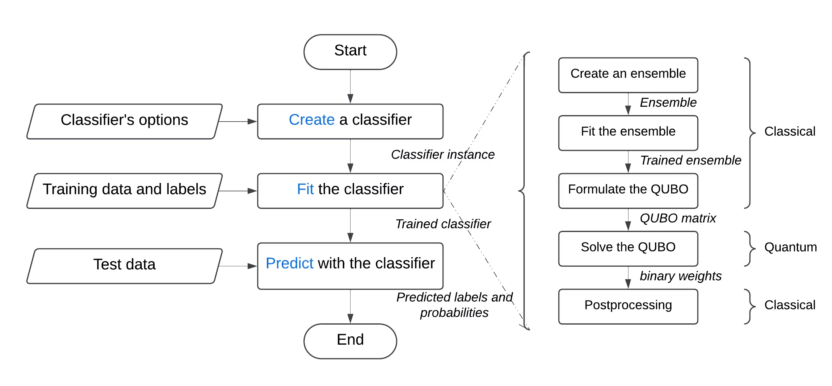
"Singularity Machine Learning - Classification" 함수를 사용하면, 양자 전문 지식 없이도 양자 하드웨어에서 실제 머신러닝 문제를 해결할 수 있습니다. 앙상블 방법 기반의 이 애플리케이션 함수는 하이브리드 분류기입니다. 초기 앙상블 훈련을 위해 부스팅, 배깅, 스태킹과 같은 고전적 방법을 활용합니다. 이후 변분 양자 고유값 솔버(VQE) 및 양자 근사 최적화 알고리즘(QAOA)과 같은 양자 알고리즘을 사용하여 훈련된 앙상블의 다양성, 일반화 능력, 전체 복잡성을 향상시킵니다.

다른 양자 머신러닝 솔루션과 달리, 이 함수는 대상 QPU의 Qubit 수에 제한받지 않고 수백만 개의 예제와 특성을 가진 대규모 데이터셋을 처리할 수 있습니다. Qubit 수는 훈련할 수 있는 앙상블의 크기만 결정합니다. 또한 매우 유연하여, 금융, 의료, 사이버 보안을 포함한 광범위한 도메인의 분류 문제를 해결하는 데 사용할 수 있습니다. 고차원, 노이즈, 불균형 데이터셋과 관련된 고전적으로 어려운 문제에서 일관되게 높은 정확도를 달성합니다. 작동 방식 다음과 같은 사용자를 위해 구축되었습니다:

양자 머신러닝을 제품 및 서비스에 통합하여 기술 제공물을 향상시키려는 기업의 엔지니어와 데이터 과학자,
양자 머신러닝 응용 프로그램을 탐색하고 분류 작업에 양자 컴퓨팅을 활용하려는 양자 연구소의 연구자, 그리고
머신러닝과 같은 과정의 교육 기관에서 양자 컴퓨팅의 장점을 시연하려는 학생과 교사.

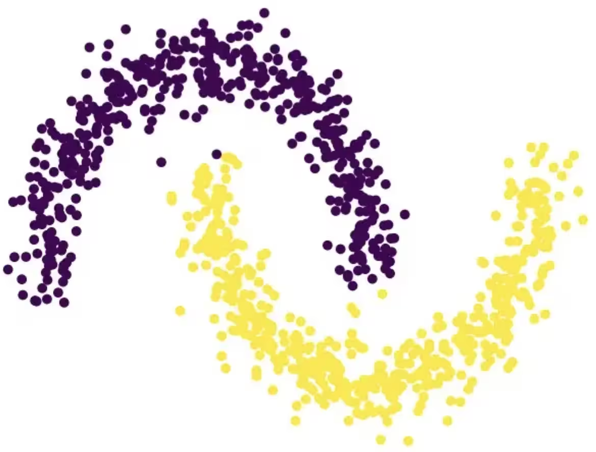
다음 예제는 create, list, fit, predict를 포함한 다양한 기능을 보여주며, 비선형 결정 경계로 인해 악명 높게 어려운 문제인 두 개의 인터리빙 반원으로 구성된 합성 문제에서의 사용법을 시연합니다.

함수 설명

이 Qiskit Function을 사용하면 Singularity의 양자 향상 앙상블 분류기를 사용하여 이진 분류 문제를 해결할 수 있습니다. 내부적으로, 레이블된 데이터셋에 대해 고전적으로 분류기 앙상블을 훈련한 다음, IBM® QPU에서 양자 근사 최적화 알고리즘(QAOA)을 사용하여 최대 다양성과 일반화를 위해 최적화하는 하이브리드 접근 방식을 사용합니다. 사용자 친화적인 인터페이스를 통해 요구 사항에 따라 분류기를 구성하고, 선택한 데이터셋에 대해 훈련하며, 이전에 보지 못한 데이터셋에 대해 예측할 수 있습니다.

일반적인 분류 문제를 해결하려면:

데이터셋을 전처리하고, 훈련 세트와 테스트 세트로 분할합니다. 선택적으로, 훈련 세트를 훈련 세트와 검증 세트로 추가 분할할 수 있습니다. scikit-learn을 사용하여 이를 수행할 수 있습니다.
훈련 세트가 불균형한 경우, imbalanced-learn을 사용하여 클래스의 균형을 맞추기 위해 리샘플링할 수 있습니다.
카탈로그의 file_upload 메서드를 사용하여 훈련, 검증, 테스트 세트를 함수의 스토리지에 개별적으로 업로드하고, 매번 관련 경로를 전달합니다.
함수의 create 액션을 사용하여 양자 분류기를 초기화합니다. 학습기의 수와 유형, 정규화(람다 값), 레이어 수, 고전적 옵티마이저 유형, 양자 Backend 등을 포함한 최적화 옵션과 같은 하이퍼파라미터를 허용합니다.
함수의 fit 액션을 사용하여 레이블된 훈련 세트(해당하는 경우 검증 세트 포함)를 전달하여 훈련 세트에서 양자 분류기를 훈련합니다.
함수의 predict 액션을 사용하여 이전에 보지 못한 테스트 세트에 대해 예측합니다.

액션 기반 접근 방식

이 함수는 액션 기반 접근 방식을 사용합니다. 액션을 사용하여 작업을 수행하거나 상태를 변경하는 가상 환경이라고 생각할 수 있습니다. 현재 다음 액션을 제공합니다: list, create, delete, fit, predict, fit_predict, create_fit_predict. 다음 예제는 create_fit_predict 액션을 시연합니다.

# Added by doQumentation — required packages for this notebook
!pip install -q numpy qiskit-ibm-catalog scikit-learn

# Import QiskitFunctionsCatalog to load the
# "Singularity Machine Learning - Classification" function by Multiverse Computing
from qiskit_ibm_catalog import QiskitFunctionsCatalog

# Import the make_moons and the train_test_split functions from scikit-learn
# to create a synthetic dataset and split it into training and test datasets
from sklearn.datasets import make_moons
from sklearn.model_selection import train_test_split

# authentication
# If you have not previously saved your credentials, follow instructions at
# /docs/guides/functions
# to authenticate with your API key.
catalog = QiskitFunctionsCatalog(channel="ibm_quantum_platform")

# load "Singularity Machine Learning - Classification" function by Multiverse Computing
singularity = catalog.load("multiverse/singularity")

# generate the synthetic dataset
X, y = make_moons(n_samples=1000)

# split the data into training and test datasets
X_train, X_test, y_train, y_test = train_test_split(X, y, test_size=0.2)

job = singularity.run(
    action="create_fit_predict",
    num_learners=10,
    regularization=0.01,
    optimizer_options={"simulator": True},
    X_train=X_train,
    y_train=y_train,
    X_test=X_test,
    options={"save": False},
)

# get job status and result
status = job.status()
result = job.result()

print("Job status: ", status)
print("Action result status: ", result["status"])
print("Action result message: ", result["message"])
print("Predictions (first five results): ", result["data"]["predictions"][:5])
print(
    "Probabilities (first five results): ",
    result["data"]["probabilities"][:5],
)
print("Usage metadata: ", result["metadata"]["resource_usage"])

Job status:  QUEUED
Action result status:  ok
Action result message:  Classifier created, fitted, and predicted.
Predictions (first five results):  [1, 0, 0, 1, 0]
Probabilities (first five results):  [[0.16849563539001172, 0.8315043646099888], [0.8726393386620336, 0.12736066133796647], [0.795344837290717, 0.20465516270928288], [0.36822585748882725, 0.6317741425111725], [0.6656662698604361, 0.3343337301395641]]
Usage metadata:  {'RUNNING: MAPPING': {'CPU_TIME': 7.945035696029663}, 'RUNNING: WAITING_QPU': {'CPU_TIME': 82.41029238700867}, 'RUNNING: POST_PROCESSING': {'CPU_TIME': 77.3459484577179}, 'RUNNING: EXECUTING_QPU': {'QPU_TIME': 71.27004957199097}}

1. List

list 액션은 공유 데이터 디렉터리에서 *.pkl.tar 형식의 저장된 모든 분류기를 검색합니다. catalog.files() 메서드를 사용하여 이 디렉터리의 내용에 접근할 수도 있습니다. 일반적으로 list 액션은 공유 데이터 디렉터리에서 *.pkl.tar 확장자를 가진 파일을 검색하고 목록 형식으로 반환합니다.

입력

Name	Type	Description	Required
`action`	`str`	The name of the action from among `create`, `list`, `fit`, `predict`, `fit_predict`, `create_fit_predict` and `delete`.	Yes

사용법

job = singularity.run(action="list")

2. Create

create 액션은 제공된 매개변수를 사용하여 지정된 quantum_classifier 유형의 분류기를 생성하고, 공유 데이터 디렉터리에 저장합니다.

참고

현재 이 함수는 QuantumEnhancedEnsembleClassifier만 지원합니다.

입력

Name	Type	Description	Required	Default
`action`	`str`	The name of the action from among `create`, `list`, `fit`, `predict`, `fit_predict`, `create_fit_predict` and `delete`.	Yes	-
`name`	`str`	The name of the quantum classifier, e.g., `spam_classifier`.	Yes	-
`instance`	`str`	IBM instance.	Yes	-
`backend_name`	`str`	IBM compute resource. Default is `None`, which means the backend with the fewest pending jobs will be used.	No	`None`
`quantum_classifier`	`str`	The type of the quantum classifier, i.e., `QuantumEnhancedEnsembleClassifier`.	No	`QuantumEnhancedEnsembleClassifier`
`num_learners`	`integer`	The number of learners in the ensemble.	No	`10`
`learners_types`	`list`	Types of learners. Among supported types are: `DecisionTreeClassifier`, `GaussianNB`, `KNeighborsClassifier`, `MLPClassifier`, and `LogisticRegression`. Further details related to each can be found in the scikit-learn documentation.	No	`[DecisionTreeClassifier]`
`learners_proportions`	`list`	Proportions of each learner type in the ensemble.	No	`[1.0]`
`learners_options`	`list`	Options for each learner type in the ensemble. For a complete list of options corresponding to the chosen learner type/s, consult scikit-learn documentation.	No	`[{"max_depth": 3, "splitter": "random", "class_weight": None}]`
`regularization_type`	`str` or `list`	Type/s of regularization to be used: `onsite` or `alpha`. `onsite` controls the onsite term where higher values lead to sparser ensembles. `alpha` controls trade-off between interaction and onsite terms where lower values lead to sparser ensembles. If a list is provided, models will be trained for each type and the best performing one will be selected.	No	`onsite`
`regularization`	`str` or `float` or `list`	Regularization value. Bounded between `0` and `+inf` if regularization_type is `onsite`. Bounded between `0` and `1` if regularization_type is `alpha`. If set to `auto`, auto-regularization is used - optimal regularization parameter is found by binary search with the desired ratio of selected classifiers to total classifiers (`regularization_desired_ratio`) and the upper bound for the regularization parameter (`regularization_upper_bound`). If a list is provided, models will be trained for each value and the best performing one will be selected.	No	`0.01`
`regularization_desired_ratio`	`float` or `list`	Desired ratio/s of selected classifiers to total classifiers for auto-regularization. If a list is provided, models will be trained for each ratio and the best performing one will be selected.	No	`0.75`
`regularization_upper_bound`	`float` or `list`	Upper bound/s for the regularization parameter when using auto-regularization. If a list is provided, models will be trained for each upper bound and the best performing one will be selected.	No	`200`
`weight_update_method`	`str`	Method for update of sample weights from among `logarithmic` and `quadratic`.	No	`logarithmic`
`sample_scaling`	`boolean`	Whether sample scaling should be applied.	No	`False`
`prediction_scaling`	`float`	Scaling factor for predictions.	No	`None`
`optimizer_options`	`dictionary`	QAOA optimizer options. A list of available options is presented later in this documentation.	No	...
`voting`	`str`	Use majority voting (`hard`) or average of probabilities (`soft`) for aggregating learners' predictions/probabilities.	No	`hard`
`prob_threshold`	`float`	Optimal probability threshold.	No	`0.5`
`random_state`	`integer`	Control randomness for repeatability.	No	`None`

추가로, optimizer_options는 다음과 같습니다:

Name	Type	Description	Required	Default
`num_solutions`	`integer`	The number of solutions	No	`1024`
`reps`	`integer`	The number of repetitions	No	`4`
`sparsify`	`float`	The sparsification threshold	No	`0.001`
`theta`	`float`	The initial value of theta, a variational parameter of QAOA	No	`None`
`simulator`	`boolean`	Whether to use a simulator or a QPU	No	`False`
`classical_optimizer`	`str`	Name of the classical optimizer for the QAOA. All solvers offered by SciPy, as enlisted here, are usable. You will need to set `classical_optimizer_options` accordingly	No	`COBYLA`
`classical_optimizer_options`	`dictionary`	Classical optimizer options. For a complete list of available options, consult SciPy documentation	No	`{"maxiter": 60}`
`optimization_level`	`integer`	The depth of the QAOA circuit	No	`3`
`num_transpiler_runs`	`integer`	Number of transpiler runs	No	`30`
`pass_manager_options`	`dictionary`	Options for generating preset pass manager	No	`{"approximation_degree": 1.0}`
`estimator_options`	`dictionary`	Estimator options. For a complete list of available options, consult Qiskit Runtime Client documentation	No	`None`
`sampler_options`	`dictionary`	Sampler options. For a complete list of available options, consult the Qiskit Runtime Client documentation	No	`None`

기본 estimator_options는 다음과 같습니다:

Name	Type	Value
`default_shots`	`integer`	`1024`
`resilience_level`	`integer`	`2`
`twirling`	`dictionary`	`{"enable_gates": True}`
`dynamical_decoupling`	`dictionary`	`{"enable": True}`
`resilience_options`	`dictionary`	`{"zne_mitigation": False, "zne": {"amplifier": "pea", "noise_factors": [1.0, 1.3, 1.6], "extrapolator": ["linear", "polynomial_degree_2", "exponential"],}}`

기본 sampler_options는 다음과 같습니다:

Name	Type	Value
`default_shots`	`integer`	`1024`
`resilience_level`	`integer`	`1`
`twirling`	`dictionary`	`{"enable_gates": True}`
`dynamical_decoupling`	`dictionary`	`{"enable": True}`

사용법

job = singularity.run(
    action="create",
    name="classifier_name",  # specify your custom name for the classifier here
    num_learners=10,
    regularization=0.01,
    optimizer_options={"simulator": True},
)

검증

name:
- 이름은 고유해야 하며, 최대 64자 길이의 문자열이어야 합니다.
- 영숫자 문자와 밑줄만 포함할 수 있습니다.
- 문자로 시작해야 하며 밑줄로 끝날 수 없습니다.
- 공유 데이터 디렉터리에 같은 이름의 분류기가 이미 존재하지 않아야 합니다.

3. Delete

delete 액션은 공유 데이터 디렉터리에서 분류기를 제거합니다.

입력

Name	Type	Description	Required
`action`	`str`	The name of the action. Must be `delete`.	Yes
`name`	`str`	The name of the classifier to delete.	Yes

사용법

job = singularity.run(
    action="delete",
    name="classifier_name",  # specify the name of the classifier to delete here
)

검증

name:
- 이름은 고유해야 하며, 최대 64자 길이의 문자열이어야 합니다.
- 영숫자 문자와 밑줄만 포함할 수 있습니다.
- 문자로 시작해야 하며 밑줄로 끝날 수 없습니다.
- 공유 데이터 디렉터리에 같은 이름의 분류기가 이미 존재해야 합니다.

4. Fit

fit 액션은 제공된 훈련 데이터를 사용하여 분류기를 훈련합니다.

입력

Name	Type	Description	Required
`action`	`str`	The name of the action. Must be `fit`.	Yes
`name`	`str`	The name of the classifier to train.	Yes
`X`	`array` or `list` or `str`	The training data. This can be a NumPy array, a list, or a string referencing a filename in the shared data directory.	Yes
`y`	`array` or `list` or `str`	The training target values. This can be a NumPy array, a list, or a string referencing a filename in the shared data directory.	Yes
`fit_params`	`dictionary`	Additional parameters to pass to the `fit` method of the classifier.	No

fit_params

Name	Type	Description	Required	Default
`validation_data`	`tuple`	The validation data and labels.	No	`None`
`pos_label`	`integer` or `str`	The class label to be mapped to 1.	No	`None`
`optimization_data`	`str`	Dataset to optimize the ensemble on. Can be one of: `train`, `validation`, `both`.	No	`train`

사용법

job = singularity.run(
    action="fit",
    name="classifier_name",  # specify the name of the classifier to train here
    X=X_train,  # or "X_train.npy" if you uploaded it in the shared data directory
    y=y_train,  # or "y_train.npy" if you uploaded it in the shared data directory
    fit_params={},  # define the fit parameters here
)

검증

name:
- 이름은 고유해야 하며, 최대 64자 길이의 문자열이어야 합니다.
- 영숫자 문자와 밑줄만 포함할 수 있습니다.
- 문자로 시작해야 하며 밑줄로 끝날 수 없습니다.
- 공유 데이터 디렉터리에 같은 이름의 분류기가 이미 존재해야 합니다.

5. Predict

predict 액션은 경성 및 연성 예측(확률)을 얻는 데 사용됩니다.

입력

Name	Type	Description	Required
`action`	`str`	The name of the action. Must be `predict`.	Yes
`name`	`str`	The name of the classifier to be used.	Yes
`X`	`array` or `list` or `str`	The test data. This can be a NumPy array, a list, or a string referencing a filename in the shared data directory.	Yes
`options["out"]`	`str`	The output JSON filename to save the predictions in the shared data directory. If not provided, the predictions are returned in the job result.	No

사용법

job = singularity.run(
    action="predict",
    name="classifier_name",  # specify the name of the classifier to use here
    X=X_test,  # or "X_test.npy" if you uploaded it to the shared data directory
    options={
        "out": "output.json",
    },
)

검증

name:
- 이름은 고유해야 하며, 최대 64자 길이의 문자열이어야 합니다.
- 영숫자 문자와 밑줄만 포함할 수 있습니다.
- 문자로 시작해야 하며 밑줄로 끝날 수 없습니다.
- 공유 데이터 디렉터리에 같은 이름의 분류기가 이미 존재해야 합니다.
options["out"]:
- 파일 이름은 고유해야 하며, 최대 64자 길이의 문자열이어야 합니다.
- 영숫자 문자와 밑줄만 포함할 수 있습니다.
- 문자로 시작해야 하며 밑줄로 끝날 수 없습니다.
- .json 확장자를 가져야 합니다.

6. Fit-predict

fit_predict 액션은 훈련 데이터를 사용하여 분류기를 훈련한 다음, 이를 사용하여 경성 및 연성 예측(확률)을 얻습니다.

입력

Name	Type	Description	Required
`action`	`str`	The name of the action. Must be `fit_predict`.	Yes
`name`	`str`	The name of the classifier to be used.	Yes
`X_train`	`array` or `list` or `str`	The training data. This can be a NumPy array, a list, or a string referencing a filename in the shared data directory.	Yes
`y_train`	`array` or `list` or `str`	The training target values. This can be a NumPy array, a list, or a string referencing a filename in the shared data directory.	Yes
`X_test`	`array` or `list` or `str`	The test data. This can be a NumPy array, a list, or a string referencing a filename in the shared data directory.	Yes
`fit_params`	`dictionary`	Additional parameters to pass to the `fit` method of the classifier.	No
`options["out"]`	`str`	The output JSON filename to save the predictions in the shared data directory. If not provided, the predictions are returned in the job result.	No

사용법

job = singularity.run(
    action="fit_predict",
    name="classifier_name",  # specify the name of the classifier to use here
    X_train=X_train,  # or "X_train.npy" if you uploaded it in the shared data directory
    y_train=y_train,  # or "y_train.npy" if you uploaded it in the shared data directory
    X_test=X_test,  # or "X_test.npy" if you uploaded it in the shared data directory
    fit_params={},  # define the fit parameters here
    options={
        "out": "output.json",
    },
)

검증

name:
- 이름은 고유해야 하며, 최대 64자 길이의 문자열이어야 합니다.
- 영숫자 문자와 밑줄만 포함할 수 있습니다.
- 문자로 시작해야 하며 밑줄로 끝날 수 없습니다.
- 공유 데이터 디렉터리에 같은 이름의 분류기가 이미 존재해야 합니다.
options["out"]:
- 파일 이름은 고유해야 하며, 최대 64자 길이의 문자열이어야 합니다.
- 영숫자 문자와 밑줄만 포함할 수 있습니다.
- 문자로 시작해야 하며 밑줄로 끝날 수 없습니다.
- .json 확장자를 가져야 합니다.

7. Create-fit-predict

create_fit_predict 액션은 분류기를 생성하고, 제공된 훈련 데이터를 사용하여 훈련한 다음, 이를 사용하여 경성 및 연성 예측(확률)을 얻습니다.

입력

Name	Type	Description	Required
`action`	`str`	The name of the action from among `create`, `list`, `fit`, `predict`, `fit_predict`, `create_fit_predict` and `delete`.	Yes
`name`	`str`	The name of the classifier to be used.	Yes
`quantum_classifier`	`str`	The type of the classifier, i.e., `QuantumEnhancedEnsembleClassifier`. Default is `QuantumEnhancedEnsembleClassifier`.	No
`X_train`	`array` or `list` or `str`	The training data. This can be a NumPy array, a list, or a string referencing a filename in the shared data directory.	Yes
`y_train`	`array` or `list` or `str`	The training target values. This can be a NumPy array, a list, or a string referencing a filename in the shared data directory.	Yes
`X_test`	`array` or `list` or `str`	The test data. This can be a NumPy array, a list, or a string referencing a filename in the shared data directory.	Yes
`fit_params`	`dictionary`	Additional parameters to pass to the `fit` method of the classifier.	No
`options["save"]`	`boolean`	Whether to save to trained classifier in the shared data directory. Default is `True`.	No
`options["out"]`	`str`	The output JSON filename to save the predictions in the shared data directory. If not provided, the predictions are returned in the job result.	No

사용법

job = singularity.run(
    action="create_fit_predict",
    name="classifier_name",  # specify your custom name for the classifier here
    num_learners=10,
    regularization=0.01,
    optimizer_options={"simulator": True},
    X_train=X_train,  # or "X_train.npy" if you uploaded it in the shared data directory
    y_train=y_train,  # or "y_train.npy" if you uploaded it in the shared data directory
    X_test=X_test,  # or "X_test.npy" if you uploaded it in the shared data directory
    fit_params={},  # define the fit parameters here
    options={
        "save": True,
        "out": "output.json",
    },
)

검증

name:
- options["save"]가 True로 설정된 경우:
  - 이름은 고유해야 하며, 최대 64자 길이의 문자열이어야 합니다.
  - 영숫자 문자와 밑줄만 포함할 수 있습니다.
  - 문자로 시작해야 하며 밑줄로 끝날 수 없습니다.
  - 공유 데이터 디렉터리에 같은 이름의 분류기가 이미 존재하지 않아야 합니다.
options["out"]:
- 파일 이름은 고유해야 하며, 최대 64자 길이의 문자열이어야 합니다.
- 영숫자 문자와 밑줄만 포함할 수 있습니다.
- 문자로 시작해야 하며 밑줄로 끝날 수 없습니다.
- .json 확장자를 가져야 합니다.

시작하기

IBM Quantum Platform API 키를 사용하여 인증하고, 다음과 같이 Qiskit Function을 선택합니다.

from qiskit_ibm_catalog import QiskitFunctionsCatalog

catalog = QiskitFunctionsCatalog(channel="ibm_quantum_platform")

# load function
singularity = catalog.load("multiverse/singularity")

예시

이 예시에서는 "Singularity Machine Learning - Classification" 함수를 사용하여 두 개의 맞물린 반원 모양(moon-shaped)으로 이루어진 데이터셋을 분류합니다. 이 데이터셋은 합성 데이터이며, 2차원으로 구성되어 있고 이진 레이블로 표시되어 있습니다. 중심점 기반 클러스터링이나 선형 분류와 같은 알고리즘에 도전적인 과제가 되도록 설계되었습니다. Moons 데이터셋 이 과정을 통해 분류기를 생성하고, 훈련 데이터에 맞게 학습시키고, 테스트 데이터에 대한 예측에 활용하며, 완료 후 분류기를 삭제하는 방법을 알아볼 수 있습니다. 시작하기 전에 scikit-learn을 설치해야 합니다. 다음 명령어를 사용하여 설치하세요.

python3 -m pip install scikit-learn

다음 단계를 수행하세요.

scikit-learn의 make_moons 함수를 사용하여 합성 데이터셋을 생성합니다.
생성된 합성 데이터셋을 공유 데이터 디렉터리에 업로드합니다.
create 액션을 사용하여 양자 강화 분류기를 생성합니다.
list 액션을 사용하여 분류기 목록을 확인합니다.
fit 액션을 사용하여 훈련 데이터로 분류기를 학습시킵니다.
predict 액션을 사용하여 학습된 분류기로 테스트 데이터를 예측합니다.
delete 액션을 사용하여 분류기를 삭제합니다.
완료 후 정리 작업을 수행합니다. Step 1. 필요한 모듈을 가져오고 합성 데이터셋을 생성한 다음, 훈련 및 테스트 데이터셋으로 분할합니다.

# import the necessary modules for this example
import os
import tarfile
import numpy as np

# Import the make_moons and the train_test_split functions from scikit-learn
# to create a synthetic dataset and split it into training and test datasets
from sklearn.datasets import make_moons
from sklearn.model_selection import train_test_split

# generate the synthetic dataset
X, y = make_moons(n_samples=10000)

# split the data into training and test datasets
X_train, X_test, y_train, y_test = train_test_split(X, y, test_size=0.2)

# print the first 10 samples of the training dataset
print("Features:", X_train[:10, :])
print("Targets:", y_train[:10])

Features: [[-0.99958218  0.02890441]
 [ 0.03285169  0.24578719]
 [ 1.13127903 -0.49134546]
 [ 1.86951286  0.00608971]
 [ 0.20190413  0.97940529]
 [ 0.8831311   0.46912627]
 [-0.10819442  0.99412975]
 [-0.20005727  0.97978421]
 [-0.78775705  0.61598607]
 [ 1.82453236 -0.0658148 ]]
Targets: [0 1 1 1 0 0 0 0 0 1]

Step 2. 레이블이 지정된 훈련 및 테스트 데이터셋을 로컬 디스크에 저장한 다음, 공유 데이터 디렉터리에 업로드합니다.

def make_tarfile(file_path, tar_file_name):
    with tarfile.open(tar_file_name, "w") as tar:
        tar.add(file_path, arcname=os.path.basename(file_path))

# save the training and test datasets on your local disk
np.save("X_train.npy", X_train)
np.save("y_train.npy", y_train)
np.save("X_test.npy", X_test)
np.save("y_test.npy", y_test)

# create tar files for the datasets
make_tarfile("X_train.npy", "X_train.npy.tar")
make_tarfile("y_train.npy", "y_train.npy.tar")
make_tarfile("X_test.npy", "X_test.npy.tar")
make_tarfile("y_test.npy", "y_test.npy.tar")

# upload the datasets to the shared data directory
catalog.file_upload("X_train.npy.tar", singularity)
catalog.file_upload("y_train.npy.tar", singularity)
catalog.file_upload("X_test.npy.tar", singularity)
catalog.file_upload("y_test.npy.tar", singularity)

# view/enlist the uploaded files in the shared data directory
print(catalog.files(singularity))

['X_test.npy.tar', 'X_train.npy.tar', 'y_test.npy.tar', 'y_train.npy.tar']

Step 3. create 액션을 사용하여 양자 강화 분류기를 생성합니다.

job = singularity.run(
    action="create",
    name="my_classifier",
    num_learners=10,
    learners_types=[
        "DecisionTreeClassifier",
        "KNeighborsClassifier",
    ],
    learners_proportions=[0.5, 0.5],
    learners_options=[{}, {}],
    regularization=0.01,
    weight_update_method="logarithmic",
    sample_scaling=True,
    optimizer_options={"simulator": True},
    voting="soft",
    prob_threshold=0.5,
)

print(job.result())

{'status': 'ok', 'message': 'Classifier created.', 'data': {}, 'metadata': {'resource_usage': {}}}

# list available classifiers using the list action
job = singularity.run(action="list")

print(job.result())

# you can also find your classifiers in the shared data directory with a *.pkl.tar extension
print(catalog.files(singularity))

{'status': 'ok', 'message': 'Classifiers listed.', 'data': {'classifiers': ['my_classifier']}, 'metadata': {'resource_usage': {}}}
['X_test.npy.tar', 'X_train.npy.tar', 'y_test.npy.tar', 'y_train.npy.tar', 'my_classifier.pkl.tar']

Step 4. fit 액션을 사용하여 양자 강화 분류기를 학습시킵니다.

job = singularity.run(
    action="fit",
    name="my_classifier",
    X="X_train.npy",  # you do not need to specify the tar extension
    y="y_train.npy",  # you do not need to specify the tar extension
)

print(job.result())

{'status': 'ok', 'message': 'Classifier fitted.', 'data': {}, 'metadata': {'resource_usage': {'RUNNING: MAPPING': {'CPU_TIME': 8.45469617843628}, 'RUNNING: WAITING_QPU': {'CPU_TIME': 69.4949426651001}, 'RUNNING: POST_PROCESSING': {'CPU_TIME': 73.01881957054138}, 'RUNNING: EXECUTING_QPU': {'QPU_TIME': 75.4787163734436}}}}

Step 5. predict 액션을 사용하여 양자 강화 분류기로부터 예측값과 확률을 구합니다.

job = singularity.run(
    action="predict",
    name="my_classifier",
    X="X_test.npy",  # you do not need to specify the tar extension
)

result = job.result()

print("Action result status: ", result["status"])
print("Action result message: ", result["message"])
print("Predictions (first five results):", result["data"]["predictions"][:5])
print(
    "Probabilities (first five results):", result["data"]["probabilities"][:5]
)

Action result status:  ok
Action result message:  Classifier predicted.
Predictions (first five results): [0, 1, 0, 0, 1]
Probabilities (first five results): [[1.0, 0.0], [0.0, 1.0], [1.0, 0.0], [1.0, 0.0], [0.0, 1.0]]

Step 6. delete 액션을 사용하여 양자 강화 분류기를 삭제합니다.

job = singularity.run(
    action="delete",
    name="my_classifier",
)

# or you can delete from the shared data directory
# catalog.file_delete("my_classifier.pkl.tar", singularity)

print(job.result())

{'status': 'ok', 'message': 'Classifier deleted.', 'data': {}, 'metadata': {'resource_usage': {}}}

Step 7. 로컬 및 공유 데이터 디렉터리를 정리합니다.

# delete the numpy files from your local disk
os.remove("X_train.npy")
os.remove("y_train.npy")
os.remove("X_test.npy")
os.remove("y_test.npy")

# delete the tar files from your local disk
os.remove("X_train.npy.tar")
os.remove("y_train.npy.tar")
os.remove("X_test.npy.tar")
os.remove("y_test.npy.tar")

# delete the tar files from the shared data
catalog.file_delete("X_train.npy.tar", singularity)
catalog.file_delete("y_train.npy.tar", singularity)
catalog.file_delete("X_test.npy.tar", singularity)
catalog.file_delete("y_test.npy.tar", singularity)

벤치마크

이 벤치마크는 분류기가 어려운 문제에서 매우 높은 정확도를 달성할 수 있음을 보여줍니다. 또한 앙상블의 학습기 수(Qubit 수)를 늘리면 정확도가 향상될 수 있음을 보여줍니다.

"고전적 정확도"는 이 경우 크기 75의 앙상블을 기반으로 하는 AdaBoost 분류기인 해당 고전적 최신 기술을 사용하여 얻은 정확도를 나타냅니다. 반면 "양자 정확도"는 "Singularity 머신 러닝 - 분류"를 사용하여 얻은 정확도를 나타냅니다.

문제	데이터셋 크기	앙상블 크기	Qubit 수	고전적 정확도	양자 정확도	개선
그리드 안정성	예제 5,000개, 특성 12개	55	55	76%	91%	15%
그리드 안정성	예제 5,000개, 특성 12개	65	65	76%	92%	16%
그리드 안정성	예제 5,000개, 특성 12개	75	75	76%	94%	18%
그리드 안정성	예제 5,000개, 특성 12개	85	85	76%	94%	18%
그리드 안정성	예제 5,000개, 특성 12개	100	100	76%	95%	19%

양자 하드웨어가 발전하고 확장됨에 따라 양자 분류기에 대한 시사점은 점점 더 중요해집니다. Qubit 수는 활용할 수 있는 앙상블의 크기에 제한을 부과하지만, 처리할 수 있는 데이터의 양을 제한하지는 않습니다. 이 강력한 기능을 통해 분류기는 수백만 개의 데이터 포인트와 수천 개의 특성을 포함하는 데이터셋을 효율적으로 처리할 수 있습니다. 중요한 점은, 앙상블 크기와 관련된 제약은 분류기의 대규모 버전 구현을 통해 해결할 수 있다는 것입니다. 반복적인 외부 루프 접근 방식을 활용하면 앙상블을 동적으로 확장하여 유연성과 전체적인 성능을 향상시킬 수 있습니다. 다만, 이 기능은 현재 버전의 분류기에는 아직 구현되지 않았습니다.

변경 로그

2025년 6월 4일

다음 업데이트와 함께 QuantumEnhancedEnsembleClassifier 업그레이드:
- 온사이트/알파 정규화 추가. regularization_type을 onsite 또는 alpha로 지정할 수 있습니다
- 자동 정규화 추가. regularization을 auto로 설정하면 자동 정규화를 사용할 수 있습니다
- 양자 최적화에 사용할 최적화 데이터를 선택하기 위해 fit 메서드에 optimization_data 매개변수 추가. train, validation, 또는 both 중 하나를 사용할 수 있습니다
- 전체적인 성능 개선
실행 중인 작업에 대한 상세 상태 추적 추가

2025년 5월 20일

오류 처리 표준화

2025년 3월 18일

qiskit-serverless를 0.20.0으로, 기본 이미지를 0.20.1로 업그레이드

2025년 2월 14일

기본 이미지를 0.19.1로 업그레이드

2025년 2월 6일

qiskit-serverless를 0.19.0으로, 기본 이미지를 0.19.0으로 업그레이드

2024년 11월 13일

Singularity 머신 러닝 - 분류 출시

지원 받기

문의 사항이 있으시면 Multiverse Computing에 문의하세요.

다음 정보를 반드시 포함해 주세요:

Qiskit Function 작업 ID (job.job_id)
문제에 대한 상세한 설명
관련 오류 메시지 또는 코드
문제를 재현하는 단계

다음 단계

권장 사항

Multiverse Computing의 Singularity 머신 러닝 분류 함수에 대한 액세스를 요청하세요.
Leclerc, L., et al. (2023). Financial risk management on a neutral atom quantum processor. Physical Review Research, 5, 043117.을 검토하세요.

개요​

함수 설명​

액션 기반 접근 방식​

1. List​

입력​

사용법​

2. Create​

입력​

사용법​

검증​

3. Delete​

입력​

사용법​

검증​

4. Fit​

입력​

fit_params​

사용법​

검증​

5. Predict​

입력​

사용법​

검증​

6. Fit-predict​

입력​

사용법​

검증​

7. Create-fit-predict​

입력​

사용법​

검증​

시작하기​

예시​

벤치마크​

변경 로그​

2025년 6월 4일​

2025년 5월 20일​

2025년 3월 18일​

2025년 2월 14일​

2025년 2월 6일​

2024년 11월 13일​

지원 받기​

다음 단계​

개요

함수 설명

액션 기반 접근 방식

1. List

입력

사용법

2. Create

입력

사용법

검증

3. Delete

입력

사용법

검증

4. Fit

입력

fit_params

사용법

검증

5. Predict

입력

사용법

검증

6. Fit-predict

입력

사용법

검증

7. Create-fit-predict

입력

사용법

검증

시작하기

예시

벤치마크

변경 로그

2025년 6월 4일

2025년 5월 20일

2025년 3월 18일

2025년 2월 14일

2025년 2월 6일

2024년 11월 13일

지원 받기

다음 단계