HI-VQE Chemistry - Qunova Computing의 Qiskit Function
# Added by doQumentation — required packages for this notebook
!pip install -q qiskit-ibm-catalog qiskit-ibm-runtime
# This cell is hidden from users
from qiskit_ibm_runtime import QiskitRuntimeService

service = QiskitRuntimeService()
instance = service.active_account()["instance"]
backend_name = service.least_busy(operational=True, min_num_qubits=16).name
API 참조를 확인하세요.
Qiskit Functions는 IBM Quantum® Premium Plan, Flex Plan, 및 On-Prem(IBM Quantum Platform API를 통한) Plan 사용자만 사용할 수 있는 실험적 기능입니다. 미리보기 릴리스 상태이며 변경될 수 있습니다.
Package versions
이 페이지의 코드는 다음 요구 사항을 사용하여 개발되었습니다. 이 버전 이상을 사용하는 것을 권장합니다.
qiskit-ibm-runtime~=0.45.0
개요
양자 화학에서 전자 구조 문제는 전자 슈뢰딩거 방정식의 해를 찾는 것에 초점을 맞춥니다 - 시스템 전자의 거동을 설명하는 양자 파동 함수입니다. 이러한 파동 함수는 복소 진폭의 벡터이며, 각 진폭은 가능한 전자 배치의 기여에 해당합니다.
기저 상태는 시스템의 가장 낮은 에너지 파동 함수이며 분자 시스템 연구에서 특별한 중요성을 가집니다. 기저 상태를 계산하는 가장 정확한 접근 방식은 가능한 모든 전자 배치를 고려하지만, 배치의 수가 시스템 크기에 따라 기하급수적으로 증가하므로 더 큰 시스템에서는 다루기 어려워집니다.
Handover Iterative Variational Quantum Eigensolver(HI-VQE)는 분자 시스템의 기저 상태를 정확하게 추정하기 위한 혁신적인 하이브리드 양자-고전 방법입니다. 양자 하드웨어와 고전 컴퓨팅을 통합하여, 양자 프로세서를 사용해 후보 전자 배치를 효율적으로 탐색하고 고전 컴퓨터에서 결과 파동 함수를 계산합니다. 간결하면서도 화학적으로 정확한 파동 함수를 생성함으로써 HI-VQE는 양자 화학 및 재료 과학의 연구와 발견을 향상시킵니다.

HI-VQE는 기저 상태를 높은 정확도로 효율적으로 추정하여 전자 구조 문제의 계산 복잡성을 줄입니다. 가장 관련성 높은 전자 배치의 신중하게 선택된 부분 집합에 초점을 맞추어 정확도와 효율성을 모두 최적화합니다.
고전 및 양자 컴퓨터의 장점을 결합하여 HI-VQE는 현재 추정 파동 함수를 반복적으로 개선합니다. 고유한 부분공간 구성 기법은 배치 선택을 더 효율적으로 만들어, 사용자가 양자 화학 시���레이션에서 더 큰 계산 제어력과 향상된 정확도를 가질 수 있게 합니다.
알고리즘에 대해 더 깊이 알고 싶다면 관련 연구 논문을 읽어보세요.
설명
분자 시스템의 전자 배치 수는 시스템 크기에 따라 기하급수적으로 증가합니다. 그러나 기저 상태와 같은 특정 전자 상태의 경우, 배치의 작은 부분만이 상태의 에너지에 크게 기여하는 것이 일반적입니다. 선택된 배치 상호작용(SCI) 방법은 이러한 희소성을 활용하여 가장 관련성 높은 배치를 식별하고 집중함으로써 계산 비용을 줄입니다. 이 배치의 부분 집합을 부분공간이라고 합니다.
HI-VQE는 분자 시스템을 표현하는 양자 컴퓨터의 고유한 효율성을 활용하여 부분공간 탐색을 지원합니다. 고전 및 양자 서브루틴을 통합하여 높은 정확도로 전자 구조 문제를 해결합니다. 기존의 양자 SCI 방법과 달리, HI-VQE는 변분 훈련, 반복적 부분공간 구성, 사전 대각화 배치 스크리닝을 결합하여 양자 측정, 반복, 고전적 대각화 비용을 줄임으로써 효율성을 향상시킵니다. 따라서 HI-VQE는 더 많은 Qubit가 필요한 더 큰 분자 시스템에 적용할 수 있으며, 동일한 정확도로 주어진 크기의 문제를 해결하는 비용을 줄입니다.
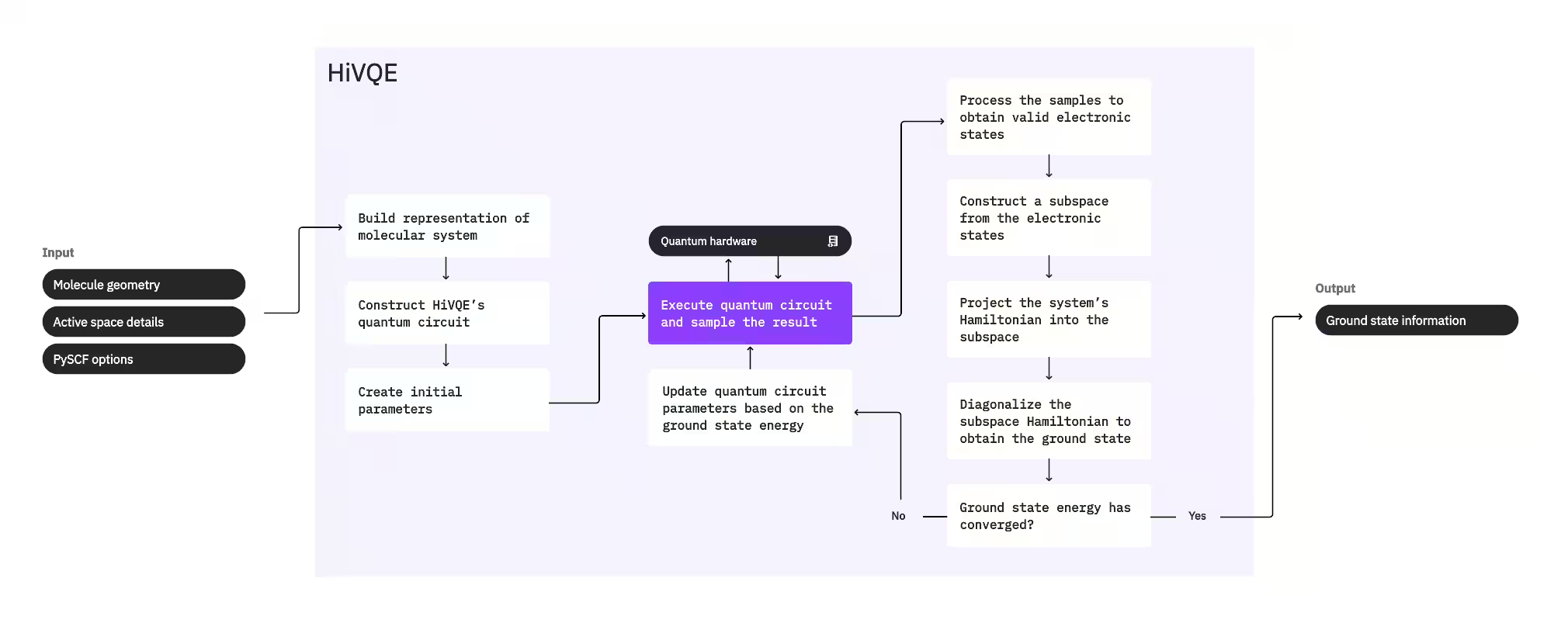
시스템의 기저 상태를 계산하기 위해, HI-VQE는 먼저 고전적 화학 패키지 PySCF를 사용하여 분자 기하학 및 기타 분자 정보와 같은 사용자 제공 입력으로부터 분자 표현을 생성합니다. 그런 다음 하이브리드 양자-고전 최적화 루프에 진입하여, 포함된 배치 수를 최소화하면서 기저 상태를 최적으로 표현하도록 부분공간을 반복적으로 개선합니다. 부분공간 크기 또는 에너지 안정성과 같은 수렴 기준이 충족될 때까지 루프가 계속된 후, 계산된 기저 상태 파동 함수와 에너지가 출력됩니다. 이러한 결과는 정확한 퍼텐셜 에너지 표면을 구성하고 시스템의 추가 분석을 수행하는 데 사용할 수 있습니다.
최적화 루프는 고품질 부분공간을 생성하기 위해 양자 회로의 매개변수를 조정하는 데 초점을 맞춥니다. HI-VQE는 세 가지 양자 회로 옵션을 제공합니다: excitation_preserving, efficient_su2, LUCJ. 최적화는 일반적인 적합성으로 인해 Hartree-Fock 참조 상태 근처에서 초기화됩니다. 그런 다음 회로가 양자 장치에서 실행되고 결과 양자 상태에서 배치가 샘플링되어 이진 문자열로 반환됩니다. 양자 장치 노이즈로 인해 일부 샘플링된 배치는 전자 수 또는 스핀을 보존하지 못하여 물리적으로 유효하지 않을 수 있습니다. HI-VQE는 qiskit-addon-sqd 패키지의 배치 복구 프로세스를 사용하여 이를 해결하므로, 사용자는 유효하지 않은 배치를 수정하거나 폐기할 수 있습니다.
유효한 배치는 최소한으로 기여할 것으로 예측되는 배치를 제거하는 선택적 스크리닝 단계를 거칩니다. 이는 부분공간의 차원을 줄여 대각화 단계의 비용을 낮춥니다. 스크리닝이 활성화된 경우, 유효한 배치에서 예비 부분공간 해밀토니안이 구성되고 매우 느슨한 종료 기준으로 대각화가 수행됩니다. 각 배치에 대한 결과 진폭의 정확도는 낮지만, 이번 반복에서 부분공간에서 제외할 배치를 예측하는 데 효과적이며 계산이 빠릅니다.
선택된 배치가 부분공간에 추가되고, 시스템의 해밀토니안이 이 부분공간에 투영됩니다. 부분공간은 반복적으로 업데이트되며, 반복 전체에서 가장 관련성 높은 배치를 보존합니다. 이 접근 방식은 양자 회로가 각 단계에서 전체 기저 상태를 근사할 필요가 없다는 점에서 대안적 방법과 대조됩니다.
다음으로, 부분공간 해밀토니안이 고전적으로 대각화되어 가장 낮은 고유값과 해당 고유벡터를 얻으며, 이는 기저 상태와 그 에너지의 근사를 나타냅니다. 반복을 통해 부분공간 품질이 향상됨에 따라, 계산된 기저 상태는 실제 기저 상태를 더 잘 근사합니다. 이 시점에서 추가 스크리닝 단계를 수행하여 계산된 기저 상태에 상당한 기여를 하지 않는 배치를 부분공간에서 제거할 수 있습니다. 이 단계는 다음 반복으로 전달되는 부분공간이 가능한 한 간결하도록 보장합니다. 이는 대각화에서 반환된 진폭을 기반으로 평가되며, 이 진폭은 계산된 기저 상태에 대한 각 배치의 중요도 기여를 나타냅니다.
그런 다음 수렴 검사에서 추가 훈련이 결과를 개선할 수 있는지 결정합니다. 그런 경우, 선택적 고전적 확장 단계가 수행되고, 양자 회로 매개변수가 계산된 에너지를 추가로 최소화하도록 업데이트되며, 프로세스가 반복됩니다. 고전적 확장 단계는 부분공간에 대한 추가 배치를 생성하여 양자 장치에서 샘플링된 배치를 보충합니다. 먼저 대각화 결과에서 가장 큰 진폭을 가진 배치를 식별한 다음, 식별된 배치에서 단일 및 이중 여기를 사용하여 새로운 배치를 생성합니다. 그런 다음 원하는 수의 이러한 배치가 부분공간에 추가됩니다.
반복이 수렴한 것으로 결정되면, HI-VQE는 계산된 기저 상태(부분공간의 상태와 기저 상태 파동 함수에서의 진폭 형태), 에너지, 그리고 계산된 상태가 시스템 해밀토니안의 고유 상태를 형성하는지 여부를 나타내는 에너지 분산 측정값을 반환합니다.
사용자는 사용할 양자 회로와 각 양자 회로에 대해 취할 샷 수를 결정할 수 있으며, 부분공간 크기를 제어하거나 양자 생성 배치를 지원하기 위한 추가 배치의 고전적 생성을 활성화할 수 있습니다. 이러한 방식으로 사용자는 원하는 애플리케이션에 맞게 HI-VQE의 동작을 맞춤 설정할 수 있습니다.
라이선스
이 Qiskit Function의 사용은 최대 20큐비트가 필요한 문제로 제한되며, 더 높은 한도를 부여하는 라이선스를 취득하지 않는 한 그러합니다.
라이선스 취득에 대해 문의하시려면 qiskit.support@qunovacomputing.com으로 이메일을 보내세요.
시작하기
먼저 함수 액세스를 요청하세요. 그런 다음 IBM Quantum® API 키를 사용하여 인증하고, 이미 계정을 저장했다고 가정하면, 다음과 같이 Qiskit Function을 선택합니다:
import reprlib
from qiskit_ibm_catalog import QiskitFunctionsCatalog

catalog = QiskitFunctionsCatalog(channel="ibm_quantum_platform")

function = catalog.load("qunova/hivqe-chemistry")
예제
첫 번째 예제는 HI-VQE 알고리즘을 사용하여 NH3 분자의 기저 상태 에너지를 계산하는 방법을 보여줍니다.
분자 기하학 및 옵션 정의
NH3의 분자 기하학은 각 원자에 대해 ";"로 구분된 데카르트 좌표로 제공됩니다.
# Define the molecule geometry
geometry = """
N         -0.85188       -0.02741        0.03141;
H          0.16545        0.00593       -0.01648;
H         -1.16348       -0.39357       -0.86702;
H         -1.16348        0.94228        0.06281;
"""
분자 시스템에 대한 추가 옵션은 다음 딕셔너리 형식으로 정의하고 제공할 수 있습니다.
# Configure some options for the job.
molecule_options = {"basis": "sto3g"}
hivqe_options = {"shots": 100, "max_iter": 20}
기하학 및 옵션 입력으로 함수를 실행합니다.
# Run HI-VQE
job = function.run(
    geometry=geometry,
    # `backend_name` is the name of a backend with at least 16 qubits,
    # for example, "ibm_marrakesh".
    backend_name=backend_name,
    max_states=2000,
    max_expansion_states=10,
    molecule_options=molecule_options,
    hivqe_options=hivqe_options,
)
문제가 발생했을 때 지원 요청에 제공할 수 있도록 Function 작업 ID를 출력하는 것이 좋습니다.
print("Job ID:", job.job_id)
Job ID: e5ced6f2-fd1d-4244-a6aa-bd27cfb0cdee
이 예제는 NH3 분자에 대해 sto3g 기저의 8개 오비탈과 16개 Qubit를 활용합니다. Qiskit Function 워크로드의 상태를 확인하거나 다음과 같이 결과를 반환합니다:
print(job.status())
QUEUED
작업이 완료된 후 result() 인스턴스로 결과를 얻을 수 있습니다.
result = job.result()

# Output can be long, so we display a shortened representation
shortened_result = reprlib.repr(result)
print(shortened_result)
{'eigenvector': [0.9824448589364075, 0.009527106392132133, 6.854074372058527e-08, 3.591500190038039e-07, 0.0012975231577544268, 2.310159709002111e-05, ...], 'energy': -55.52108557170985, 'energy_history': [-55.51901898989887, -55.52056881448526, -55.52065046778772, -55.520690696813716, -55.520691108428, -55.520708448092634, ...], 'energy_variance': 3.066239097617371e-10, ...}
기저 상태 에너지에 접근하려면 "energy" 키를 사용하세요. "eigenvector" 키는 결과의 "states"에 저장된 전자 배치의 해당 비트스트링 표기법과 함께 CI 계수를 제공합니다.
fci_energy = -55.521148034704126  # the exact energy using FCI method
hivqe_energy = result["energy"]
print(
    f"|Exact Energy - HI-VQE Energy|: "
    f"{abs(fci_energy - hivqe_energy) * 1000} mHa"
)
print(f"Sampled Number of States: {len(result['states'])}")
|Exact Energy - HI-VQE Energy|: 0.06246299427914437 mHa
Sampled Number of States: 1936
성능
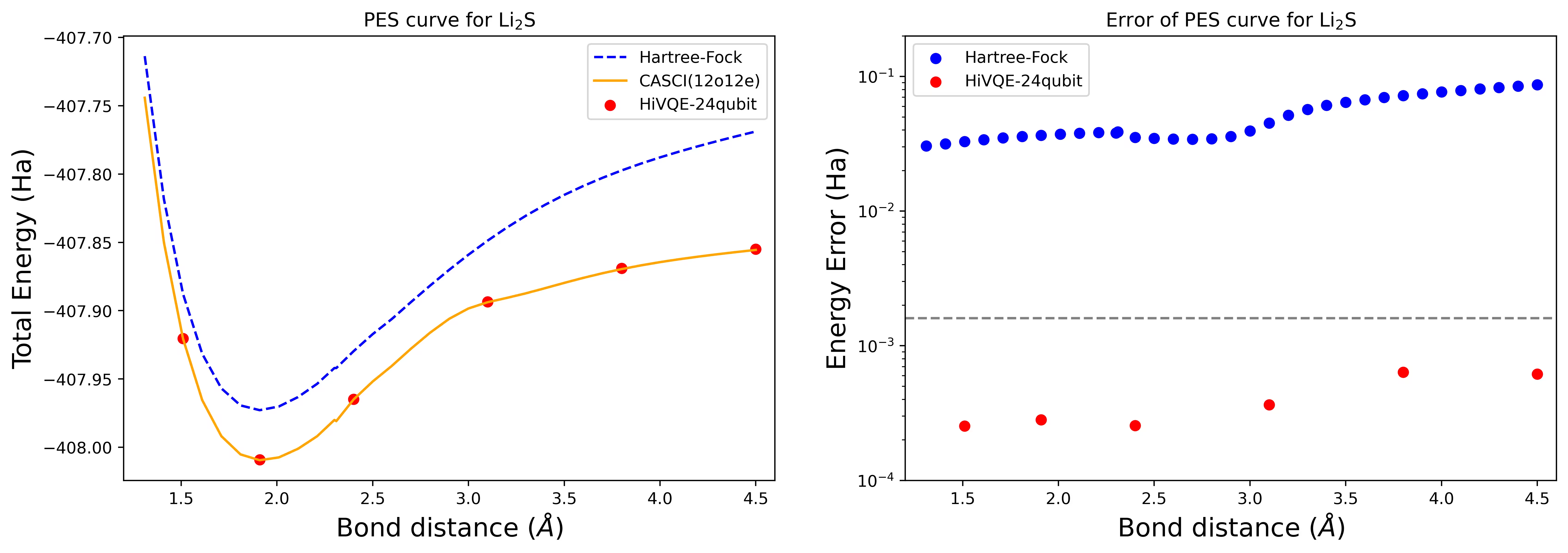
이 섹션에서는 Li2S에 대한 24-Qubit 케이스, N2 분자에 대한 40-Qubit 케이스, FeP-NO 시스템에 대한 44-Qubit 케이스로 시연된 HI-VQE의 벤치마크 계산을 보여줍니다.
24 qubit Li2S 분자의 해리 퍼텐셜 에너지 표면 곡선
PES 곡선은 FCI 참조 및 RHF의 초기 추정과 함께 FCI 참조로부터의 에너지 오차와 함께 표시됩니다.
계산은 다음 기하학 및 옵션으로 수행되었습니다.
# This cell is hidden from users
backend_name = service.least_busy(operational=True, min_num_qubits=38).name
# Define Li2S geometries
Li2S_geoms = {
    "Li2S_1.51": "S        -1.239044    0.671232   -0.030374;Li       -1.506327    0.432403   -1.498949;Li       -0.899996    0.973348    1.826768;",
    "Li2S_2.40": "S        -1.741432    0.680397    0.346702;Li       -0.529307    0.488006   -1.729343;Li       -1.284307    0.989409    2.177209;",
    "Li2S_3.80": "S        -2.707255    0.674298    0.909161;Li        0.079218    0.552012   -1.671656;Li       -0.927010    0.931502    1.557063;",
}

# Configure some options for the job.
molecule_options = {
    "basis": "sto3g",
}
hivqe_options = {
    "shots": 100,
    "max_iter": 20,
}

results = []
for geom in ["Li2S_1.51", "Li2S_2.40", "Li2S_3.80"]:
    # Run HI-VQE
    job = function.run(
        geometry=Li2S_geoms[geom],
        backend_name=backend_name,  # can use any device with at least 38 qubits
        max_states=2000,
        max_expansion_states=10,
        molecule_options=molecule_options,
        hivqe_options=hivqe_options,
    )
    results.append(job.result())
빨간 점은 6개의 서로 다른 기하학에 대한 HI-VQE 계산 결과를 나타내며, 1.51, 2.40, 3.80 Angstrom에 해당하는 세 가지 기하학이 위 셀에서 입력으로 제공됩니다.
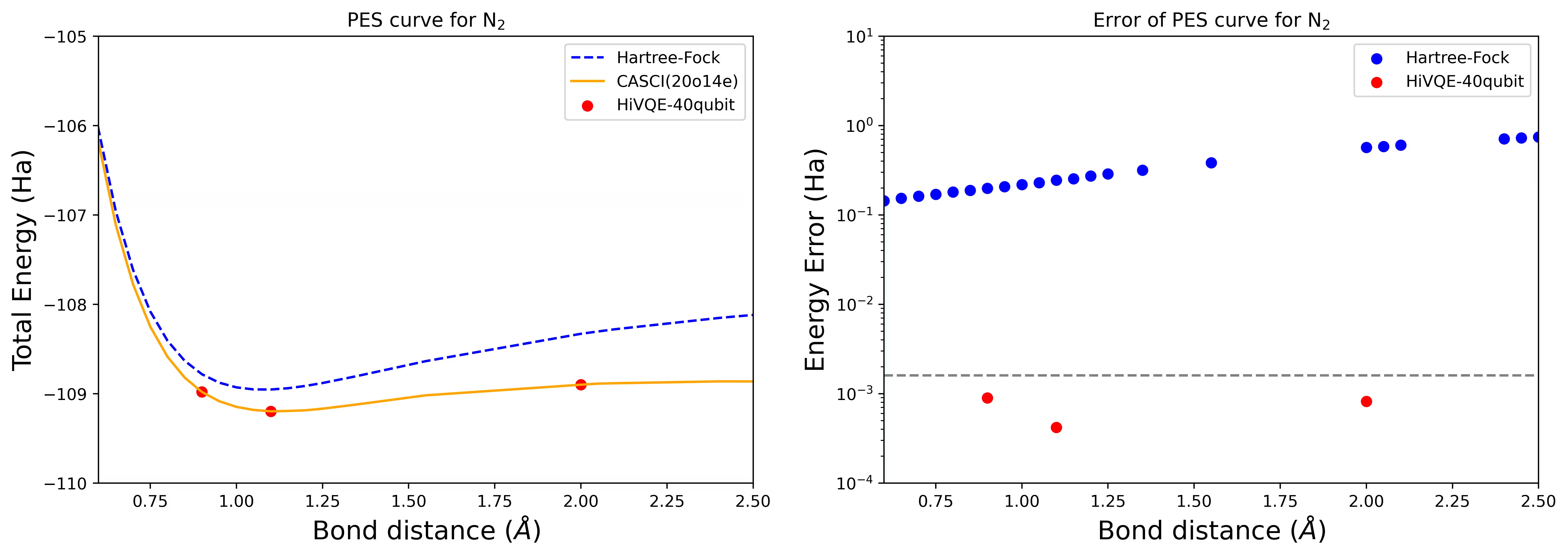
40 qubit N2 분자의 해리 PES 곡선
질소 분자는 Hartree-Fock 상태를 넘어서는 큰 상관 에너지 기여를 가진 다중참조 시스템으로 확인되었습니다. cc-pvdz 기저, (20o,14e)를 사용하여 homo-lumo 활성 오비탈 선택으로 N2 분자에 대한 벤치마크 계산을 수행했습니다. 이 문제를 나타내는 완전 활성 공간(CAS) 수는 6,009,350,400입니다. 강력한 데스크톱(16cpu/64GB)에서 이 수의 상태로 고유값 문제 해(에너지 및 전자 구조에 대한)를 얻는 것은 불가능합니다. HI-VQE를 사용하면 사용자는 CAS 상태의 부분공간을 효율적으로 탐색하여 계산 리소스를 크게 절약하면서 화학적으로 정확한 결과를 찾을 수 있습니다. 다음 플롯은 N2 분자 해리의 40 qubit HI-VQE 계산의 PES 곡선을 보여줍니다.
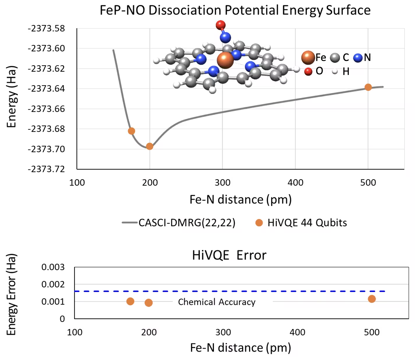
44 qubit FeP-NO 시스템의 5배위 철(II)-포르피린 해리 PES 곡선
또 다른 흥미로운 화학 시스템은 배위된 일산화질소(NO) 리간드를 가진 철(II)-포르피린(FeP) 복합체로, 다양한 생리적 과정에서 중요한 역���을 하는 생물학적으로 관련된 금속포르피린 시스템을 나타냅니다. 이 예제에서는 HI-VQE를 활용하여 FeP와 NO 간의 분자간 상호작용의 정확한 퍼텐셜 에너지 표면 곡선(서로 다른 분리 기하학에 대한 기저 상태 에너지)을 추정했습니다. 결합된 시스템은 총 6-31g(d) 기저로 450개의 오비탈과 202개의 전자(450o,202e)를 가집니다. homo-lumo 활성 오비탈 선택을 활용��여 실제 케이스에서 (22o,22e)의 더 작은 케이스를 계산했습니다. 다음 벤치마크 결과에서, 최첨단 고전적 컴퓨터 화학 계산인 CASCI(DMRG) (22o,22e) 참조와의 화학적 정확도(> 1.6 mHa)를 달성할 수 있었습니다.
벤치마크
- 정확한 행렬 크기는 FCI 및 CASCI와 같은 정확한 해에 대한 행렬식의 수입니다.
- HI-VQE 계산은 그 부분공간을 샘플링하고 계산합니다(즉, HI-VQE 행렬 크기).
- 총 시간에는 QPU 런타임과 CPU를 사용한 Qiskit Function 실행이 포함됩니다.
- 정확도는 정확한 해와의 에너지 차이로 추정됩니다.
| Chemical system | Number of qubits | Exact matrix size | HI-VQE matrix size | E(diff) from exact (mHa) | Number of iteration | Total time | QPU runtime usage |
|---|---|---|---|---|---|---|---|
| (8o,10e) | 16 | 3136 | 1936 | 0.08 | 6 | 37 s | 34 s |
| (10o,10e) | 20 | 63504 | 3969 | 0.60 | 5 | 250 s | 50 s |
| (15o,10e) | 30 | 9018009 | 49729 | 0.90 | 5 | 354 s | 54 s |
| (16o,14e) | 32 | 130873600 | 1798281 | 1.10 | 9 | 6531 s | 121 s |
| (18o,24e) | 36 | 344622096 | 399424 | 0.90 | 24 | 5174 s | 130 s |
| (20o,14e) | 40 | 6009350400 | 9012004 | 1.20 | 21 | 46547 s | 258 s |
오류 메시지 가져오기
워크로드가 실패하면 상태가 ERROR가 되고 job.result()를 호출하면 예외가 발생합니다:
job = function.run(
    geometry="invalid-geometry",  # This will cause an error
    backend_name=backend_name,
    max_states=2000,
    max_expansion_states=15,
    molecule_options=molecule_options,
    hivqe_options=hivqe_options,
)

job.result()
job.status()
'ERROR'
지원 받기
이 함수에 대한 도움을 받으려면 qiskit.support@qunovacomputing.com으로 이메일을 보내세요.
특정 오류의 문제 해결에 대한 도움이 필요하면 오류가 발생한 작업의 Function 작업 ID를 제공하세요.
다음 단계
- 이 양식을 작성하여 함수 액세스를 요청하세요.
- 이 Qiskit Function의 API 참조를 방문하세요.
- HI-VQE로 FeP-NO의 해리 PES 곡선 계산 튜토리얼을 시도해 보세요.
- Pellow-Jarman, A., et al. (2025). HIVQE: Handover Iterative Variational Quantum Eigensolver for Efficient Quantum Chemistry Calculations. arXiv preprint arXiv:2503.06292.를 검토하세요.
- Qunova HiVQE를 사용한 해리 PES 곡선 튜토리얼을 시도해 보세요.