파울리 연산자 투영 벤치마크

계산 기저 상태에 대한 파울리 문자열의 작용

계산 기저 상태에 대한 파울리 문자열의 작용은 상당히 단순하며, 그 결과 자체가 하나의 계산 기저 상태입니다. 이는 파울리 행렬의 구조, 즉 각 행에 0이 아닌 원소가 하나만 있다는 사실에서 직접 나오는 결과입니다. 따라서 Qubit에 대한 작용은 다음과 같습니다:

\sigma_x |0 \rangle = |1 \rangle

\sigma_x |1 \rangle = |0 \rangle

\sigma_y |0 \rangle = i|1 \rangle

\sigma_y |1 \rangle = -i|0 \rangle

\sigma_z |0 \rangle = |0 \rangle

\sigma_z |1 \rangle = -|1 \rangle

I |0 \rangle = |0 \rangle

I |1 \rangle = |1 \rangle

계산 기저를 나타내는 비트열의 각 비트는 $x \in \{0, 1 \}$ 로 표기합니다. 구현을 최대한 가볍게 유지하기 위해 비트열을 bool 변수로 표현합니다: $0\rightarrow \textrm{False}$ , $1\rightarrow \textrm{True}$ .

각 파울리 연산자가 계산 기저 상태에 미치는 작용을 나타내기 위해 세 개의 변수 diag, sign, imag를 할당합니다.

diag는 연산자가 대각인지 여부를 나타냅니다:
- $\textrm{diag}(I) = \textrm{True}$
- $\textrm{diag}(\sigma_x) = \textrm{False}$
- $\textrm{diag}(\sigma_y) = \textrm{False}$
- $\textrm{diag}(\sigma_z) = \textrm{True}$
sign은 0 또는 1에 연결된 행렬 원소에 부호 변화가 있는지를 나타냅니다:
- $\textrm{sign}(I) = \textrm{False}$
- $\textrm{sign}(\sigma_x) = \textrm{False}$
- $\textrm{sign}(\sigma_y) = \textrm{True}$
- $\textrm{sign}(\sigma_z) = \textrm{True}$
imag는 행렬 원소에 복소수 성분이 있는지를 나타냅니다:
- $\textrm{imag}(I) = \textrm{False}$
- $\textrm{imag}(\sigma_x) = \textrm{False}$
- $\textrm{imag}(\sigma_y) = \textrm{True}$
- $\textrm{imag}(\sigma_z) = \textrm{False}$

임의의 파울리 연산자를 $\sigma \in \{ I, \sigma_x, \sigma_y \sigma_z\}$ 로 표기합니다. 그러면 파울리 연산자가 계산 기저 상태에 미치는 작용은 다음 논리 연산으로 나타낼 수 있습니다:

\sigma |x \rangle = |x == \textrm{diag}(\sigma) \rangle (-1)^{x\textrm{ and sign}(\sigma)} (i)^{\textrm{imag}(\sigma)}.

이는 임의의 Qubit 수로도 간단히 일반화됩니다. 실제로 동작하는지 확인해 보겠습니다:

# Added by doQumentation — installs the packages this notebook needs if they are missing
import importlib.util

_needed = {"matplotlib": "matplotlib", "numpy": "numpy", "qiskit": "qiskit", "qiskit_addon_sqd": "qiskit-addon-sqd"}
_missing = [pip for module, pip in _needed.items()
            if importlib.util.find_spec(module) is None]
# One at a time, so a package that fails to install does not block the others
for _pip in _missing:
    %pip install -q {_pip}
if not _missing:
    print("\u2713 All required packages are installed")

def connected_element_and_amplitude_bool(
    x: bool, diag: bool, sign: bool, imag: bool
) -> tuple[bool, complex]:
    """
    Finds the connected element to computational basis state |x> under
    the action of the Pauli operator represented by (diag, sign, imag).

    Args:
        x: Value of the bit, either True or False.
        diag: Whether the Pauli operator is diagonal (I, Z)
        sigma: Whether the Pauli operator's rows differ in sign (Y, Z)
        imag: Whether the Pauli operator is purely imaginary (Y)

    Returns:
        A length-2 tuple:
            - The connected element to x, either False or True
            - The matrix element
    """
    return x == diag, (-1) ** (x and sign) * (1j) ** (imag)

sigma_indices = [0, 1, 2, 3]
sigma_string = ["I", "SX", "SZ", "SY"]
sigma_diag = [True, False, True, False]
sigma_sign = [False, False, True, True]
sigma_imag = [False, False, False, True]
qubit_values = [False, True]

for xi in sigma_indices:
    print("-------------------")
    print(sigma_string[xi])
    for x in qubit_values:
        x_p, matrix_element = connected_element_and_amplitude_bool(
            x, sigma_diag[xi], sigma_sign[xi], sigma_imag[xi]
        )
        print(
            "|"
            + str(x)
            + "> -->  |"
            + str(x_p)
            + ">    ME:"
            + str(matrix_element)
        )

-------------------
I
|False> -->  |False>    ME:(1+0j)
|True> -->  |True>    ME:(1+0j)
-------------------
SX
|False> -->  |True>    ME:(1+0j)
|True> -->  |False>    ME:(1+0j)
-------------------
SZ
|False> -->  |False>    ME:(1+0j)
|True> -->  |True>    ME:(-1+0j)
-------------------
SY
|False> -->  |True>    ME:1j
|True> -->  |False>    ME:(-0-1j)

40 Qubit 시스템에 대해 많은 수(5천만 개)의 비트열을 생성합니다:

import numpy as np
from qiskit_addon_sqd.qubit import sort_and_remove_duplicates

rand_seed = 22
np.random.seed(rand_seed)

# Generate some random bitstrings for testing

def random_bitstrings(n_samples, n_qubits):
    return (
        np.round(np.random.rand(n_samples, n_qubits))
        .astype("int")
        .astype("bool")
    )

n_qubits = 40
bts_matrix = random_bitstrings(50_000_000, n_qubits)

# We need to sort the bitstrings and only keep the unique ones
# NOTE: It is essential for the projection code to have the bitstrings sorted!
bts_matrix = sort_and_remove_duplicates(bts_matrix).astype("bool")

# Final subspace dimension after getting rid of duplicated bitstrings
d = bts_matrix.shape[0]

print("Total number of unique bitstrings: " + str(d))

Total number of unique bitstrings: 49998839

SQD 파울리 투영 함수 벤치마크

고려하는 파울리 문자열은 $\sigma_z \otimes ... \otimes \sigma_z$ 입니다.

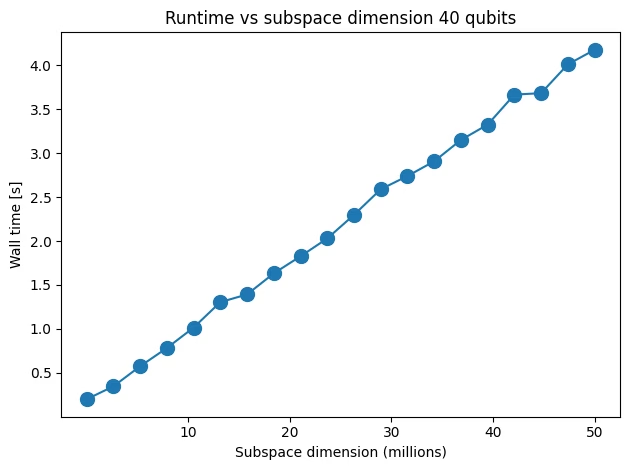
비트열 행렬을 슬라이싱하여 서로 다른 부분 공간 차원을 고려합니다. 부분 공간 크기별로 부분 공간 투영 시간을 측정합니다.

import time

from qiskit.quantum_info import Pauli
from qiskit_addon_sqd.qubit import matrix_elements_from_pauli

pauli = Pauli("Z" * n_qubits)

# Different subspace sizes to test
d_list = np.linspace(d / 1000, d, 20).astype("int")

# To store the walltime
time_array = np.zeros(20)

for i in range(20):
    int_bts_matrix = bts_matrix[: d_list[i], :]
    time_1 = time.time()
    _ = matrix_elements_from_pauli(int_bts_matrix, pauli)
    time_array[i] = time.time() - time_1
    print(f"Iteration {i} took {round(time_array[i], 6)}s")

Iteration 0 took 0.201246s
Iteration 1 took 0.348222s
Iteration 2 took 0.576333s
Iteration 3 took 0.78356s
Iteration 4 took 1.016162s
Iteration 5 took 1.305325s
Iteration 6 took 1.392751s
Iteration 7 took 1.632433s
Iteration 8 took 1.826521s
Iteration 9 took 2.02903s
Iteration 10 took 2.297458s
Iteration 11 took 2.588042s
Iteration 12 took 2.738746s
Iteration 13 took 2.906144s
Iteration 14 took 3.148833s
Iteration 15 took 3.323253s
Iteration 16 took 3.664171s
Iteration 17 took 3.680663s
Iteration 18 took 4.008313s
Iteration 19 took 4.173532s

import matplotlib.pyplot as plt

# Data for energies plot
x1 = d_list
y1 = time_array

# Plot energies
plt.title("Runtime vs subspace dimension 40 qubits")
plt.xlabel("Subspace dimension (millions)")
plt.ylabel("Wall time [s]")
plt.xticks([1e7, 2e7, 3e7, 4e7, 5e7], [str(i) for i in [10, 20, 30, 40, 50]])
plt.plot(x1, y1, marker=".", markersize=20)
plt.tight_layout()
plt.show()

Output of the previous code cell

이제 60 Qubit에 대해 같은 작업을 수행합니다:

n_qubits = 60
bts_matrix = random_bitstrings(50_000_000, n_qubits)

# We need to sort the bitstrings and just keep the unique ones
bts_matrix = sort_and_remove_duplicates(bts_matrix).astype("bool")

# Final subspace dimension after getting rid of duplicated bitstrings
d = bts_matrix.shape[0]

print("Total number of unique bitstrings: " + str(d))

Total number of unique bitstrings: 50000000

pauli = Pauli("Z" * n_qubits)

# Different subspace sizes to test
d_list = np.linspace(d / 1000, d, 20).astype("int")

# It is better to do this once
row_array = np.arange(d)

# To store the walltime
time_array = np.zeros(20)

for i in range(20):
    int_bts_matrix = bts_matrix[: d_list[i], :]
    int_row_array = row_array[: d_list[i]]
    time_1 = time.time()
    _ = matrix_elements_from_pauli(int_bts_matrix, pauli)
    time_array[i] = time.time() - time_1
    print(f"Iteration {i} took {round(time_array[i], 6)}s")

Iteration 0 took 0.236567s
Iteration 1 took 0.424116s
Iteration 2 took 0.673399s
Iteration 3 took 0.905164s
Iteration 4 took 1.168936s
Iteration 5 took 1.454204s
Iteration 6 took 1.74778s
Iteration 7 took 1.920795s
Iteration 8 took 2.259994s
Iteration 9 took 2.550674s
Iteration 10 took 2.681287s
Iteration 11 took 3.04411s
Iteration 12 took 3.293262s
Iteration 13 took 3.471247s
Iteration 14 took 3.726639s
Iteration 15 took 4.072854s
Iteration 16 took 4.221037s
Iteration 17 took 4.498535s
Iteration 18 took 4.741108s
Iteration 19 took 5.159038s

# Data for energies plot
x1 = d_list
y1 = time_array

fig, axs = plt.subplots(1, 1, figsize=(6, 6))

# Plot energies
axs.plot(x1, y1, marker=".", markersize=20)
axs.set_title("Runtime vs subspace dimension 60 qubits")
axs.set_xlabel("Subspace dimension (millions)")
plt.xticks([1e7, 2e7, 3e7, 4e7, 5e7], [str(i) for i in [10, 20, 30, 40, 50]])
axs.set_ylabel("Wall time [s]")

plt.tight_layout()
plt.show()

Output of the previous code cell

계산 기저 상태에 대한 파울리 문자열의 작용​

SQD 파울리 투영 함수 벤치마크​

계산 기저 상태에 대한 파울리 문자열의 작용

SQD 파울리 투영 함수 벤치마크