부분 공간 차원 제한
이 안내서에서는 자기 일관적 구성 복구 기법에서 부분 공간 차원이 미치는 효과를 보여 드립니다.
선험적으로, 목표 정확도를 얻으려면 부분 공간 차원이 얼마여야 하는지 알 수 없습니다. 그러나 부분 공간 차원을 늘리면 방법의 정확도가 높아진다는 것은 알고 있습니다. 따라서 부분 공간 차원의 함수로서 예측의 정확도를 살펴볼 수 있습니다. 분자와 그 속성을 지정합니다.
# Added by doQumentation — installs the packages this notebook needs if they are missing
import importlib.util

_needed = {"matplotlib": "matplotlib", "numpy": "numpy", "pyscf": "pyscf", "qiskit_addon_sqd": "qiskit-addon-sqd"}
_missing = [pip for module, pip in _needed.items()
            if importlib.util.find_spec(module) is None]
# One at a time, so a package that fails to install does not block the others
for _pip in _missing:
    %pip install -q {_pip}
if not _missing:
    print("\u2713 All required packages are installed")
import warnings

import pyscf
import pyscf.cc
import pyscf.mcscf

warnings.filterwarnings("ignore")

# Specify molecule properties
open_shell = False
spin_sq = 0

# Build N2 molecule
mol = pyscf.gto.Mole()
mol.build(
    atom=[["N", (0, 0, 0)], ["N", (1.0, 0, 0)]],
    basis="6-31g",
    symmetry="Dooh",
)

# Define active space
n_frozen = 2
active_space = range(n_frozen, mol.nao_nr())

# Get molecular integrals
scf = pyscf.scf.RHF(mol).run()
num_orbitals = len(active_space)
n_electrons = int(sum(scf.mo_occ[active_space]))
num_elec_a = (n_electrons + mol.spin) // 2
num_elec_b = (n_electrons - mol.spin) // 2
cas = pyscf.mcscf.CASCI(scf, num_orbitals, (num_elec_a, num_elec_b))
mo = cas.sort_mo(active_space, base=0)
hcore, nuclear_repulsion_energy = cas.get_h1cas(mo)
eri = pyscf.ao2mo.restore(1, cas.get_h2cas(mo), num_orbitals)

# Compute exact energy
exact_energy = cas.run().e_tot
converged SCF energy = -108.835236570775
CASCI E = -109.046671778080  E(CI) = -32.8155692383188  S^2 = 0.0000000
QPU 샘플을 대신할 무작위 비트열을 생성합니다.
import numpy as np
from qiskit_addon_sqd.counts import generate_bit_array_uniform

# Create a seed to control randomness throughout this workflow
rng = np.random.default_rng(24)

# Generate random samples
bit_array = generate_bit_array_uniform(
    10_000, num_orbitals * 2, rand_seed=rng
)
배치 크기를 늘려 가며 SQD를 호출합니다.
from qiskit_addon_sqd.fermion import diagonalize_fermionic_hamiltonian

list_samples_per_batch = [50, 200, 400, 600]

# SQD options
max_iterations = 5

# Eigenstate solver options
num_batches = 10
max_davidson_cycles = 200

energies = []
subspace_dimensions = []

for samples_per_batch in list_samples_per_batch:
    result = diagonalize_fermionic_hamiltonian(
        hcore,
        eri,
        bit_array,
        samples_per_batch=samples_per_batch,
        norb=num_orbitals,
        nelec=(num_elec_a, num_elec_b),
        num_batches=num_batches,
        max_iterations=max_iterations,
        symmetrize_spin=True,
        seed=rng,
    )
    energies.append(result.energy)
    subspace_dimensions.append(np.prod(result.sci_state.amplitudes.shape))
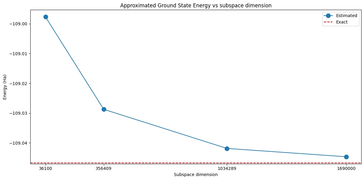
이 그래프는 부분 공간 차원을 늘리면 더 정확한 결과가 나온다는 것을 보여 줍니다.
import matplotlib.pyplot as plt

# Data for energies plot
x1 = subspace_dimensions
y1 = np.array(energies) + nuclear_repulsion_energy

fig, axs = plt.subplots(1, 1, figsize=(12, 6))

# Plot energies
axs.plot(x1, y1, marker=".", markersize=20, label="Estimated")
axs.set_xticks(x1)
axs.set_xticklabels(x1)
axs.axhline(y=exact_energy, color="red", linestyle="--", label="Exact")
axs.set_title("Approximated Ground State Energy vs subspace dimension")
axs.set_xlabel("Subspace dimension")
axs.set_ylabel("Energy (Ha)")
axs.legend()

plt.tight_layout()
plt.show()
max_dim으로 명시적 한계 설정하기
위의 스윕에서는 부분 공간 차원이 간접적으로만 제어되었습니다. samples_per_batch는 각 배치에 몇 개의 비트열을 뽑을지 정하지만, 결과 부분 공간의 차원은 그 비트열에 포함된 서로 다른 스핀 알파 및 스핀 베타 문자열의 수에 의해 결정되며, 서브샘플링에 사용할 수 있는 구성 풀은 구성 복구 반복이 진행될수록 커집니다. 그래서 위 가로축의 부분 공간 차원은 우리가 고르지 않은 불규칙한 숫자입니다.
diagonalize_fermionic_hamiltonian의 max_dim 인수는 차원을 직접 제한합니다. 이 인수는 각 스핀 섹터에 유지되는 CI 문자열의 수를 제한하며, 부분 공간은 두 섹터의 데카르트 곱으로 생성되므로 그 차원은 두 섹터 차원의 곱입니다:
-
max_dim=d는 두 섹터를 모두d개의 문자열로 제한하므로, 부분 공간 차원은 최대d ** 2입니다. -
max_dim=(d_a, d_b)는 스핀 알파와 스핀 베타 섹터를 따로 제한하므로, 부분 공간 차원은 최대d_a * d_b입니다.symmetrize_spin=True일 때는 두 한계가 같아야 합니다. -
기본값인
max_dim=None은 제한을 두지 않습니다.
배치에 한계보다 많은 문자열이 있으면 가장 덜 중요한 것부터 버려집니다. include_configurations로 전달한 문자열이 먼저 유지되고, 그다음 이전 반복에서 이월된 문자열(carryover_threshold 참고)이 유지되며, 남은 자리는 샘플링된 횟수가 많은 순서대로 샘플링된 문자열로 채워집니다.
max_dim은 고유 상태 솔버가 수행해야 하는 가장 큰 대각화의 크기에 상한을 두므로, 솔버를 런타임과 메모리 예산 안에 유지하는 편리한 방법입니다. samples_per_batch는 넉넉하게 선택하고, 부분 공간이 얼마나 커질 수 있는지는 max_dim이 결정하게 하세요.
아래에서는 samples_per_batch를 고정하고 max_dim을 늘려 가며 연구를 반복합니다.
list_max_dim = [100, 200, 400, 800]

# Use a generous number of samples per batch, so that max_dim is what limits
# the dimension of the subspace
samples_per_batch = 600

energies_max_dim = []
subspace_dimensions_max_dim = []

for max_dim in list_max_dim:
    result = diagonalize_fermionic_hamiltonian(
        hcore,
        eri,
        bit_array,
        samples_per_batch=samples_per_batch,
        norb=num_orbitals,
        nelec=(num_elec_a, num_elec_b),
        num_batches=num_batches,
        max_iterations=max_iterations,
        symmetrize_spin=True,
        max_dim=max_dim,
        seed=rng,
    )
    energies_max_dim.append(result.energy)
    subspace_dimensions_max_dim.append(
        int(np.prod(result.sci_state.amplitudes.shape))
    )

print(f"max_dim:            {list_max_dim}")
print(f"subspace dimension: {subspace_dimensions_max_dim}")
max_dim:            [100, 200, 400, 800]
subspace dimension: [10000, 40000, 160000, 640000]
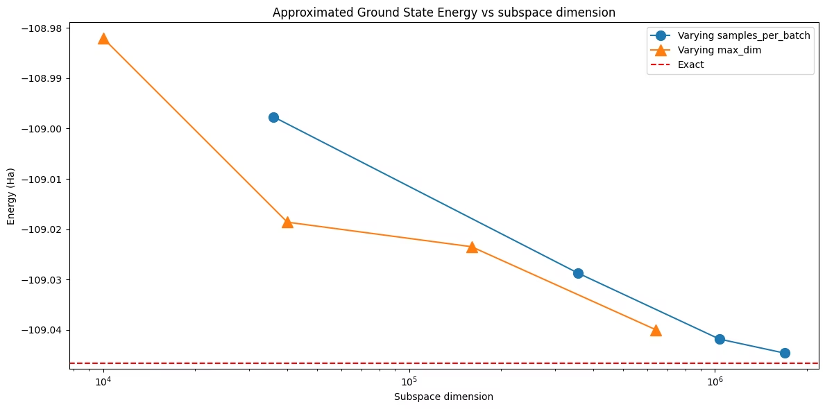
이제 부분 공간 차원은 모든 실행에서 정확히 max_dim ** 2입니다. 발견된 것이 아니라 선택된 값입니다. 두 스윕을 함께 그려 보면 어느 인수로 그 차원에 도달했든 정확도는 부분 공간 차원 자체에 의해 좌우된다는 것을 알 수 있습니다. 다만 두 곡선이 정확히 일치할 필요는 없습니다. max_dim 실행은 배치당 600개의 비트열을 뽑은 다음 가장 자주 샘플링된 문자열을 유지하므로, 같은 차원에서 처음부터 더 적은 비트열을 샘플링하여 그 차원에 도달한 실행보다 더 좋은 구성 집합을 유지할 수 있습니다.
fig, axs = plt.subplots(1, 1, figsize=(12, 6))

axs.plot(
    subspace_dimensions,
    np.array(energies) + nuclear_repulsion_energy,
    marker=".",
    markersize=20,
    label="Varying samples_per_batch",
)
axs.plot(
    subspace_dimensions_max_dim,
    np.array(energies_max_dim) + nuclear_repulsion_energy,
    marker="^",
    markersize=12,
    label="Varying max_dim",
)
axs.axhline(y=exact_energy, color="red", linestyle="--", label="Exact")
axs.set_xscale("log")
axs.ticklabel_format(axis="y", useOffset=False)
axs.set_title("Approximated Ground State Energy vs subspace dimension")
axs.set_xlabel("Subspace dimension")
axs.set_ylabel("Energy (Ha)")
axs.legend()

plt.tight_layout()
plt.show()