비마르코프 오류 검사를 사용한 사후 선택

이 가이드는 비마르코프 오류 검사가 무엇인지, 그리고 qiskit-mitigation으로 이를 소프트웨어에서 어떻게 구현하는지 설명합니다. 먼저 Qubit 2개의 작은 예제로 검사를 시각화하고 작동 방식을 논의합니다. 감을 익힌 후에는 20 Qubit 예제에서 검사를 구현하고 여러 사후 선택 전략을 비교해 봅니다.

비마르코프 오류 검사란 무엇인가요?

비마르코프 오류 검사는 Qubit의 상태가 비마르코프 오류원에 의해 손상되었을 가능성이 있는지 측정으로 확인하는 테스트입니다. 이 테스트는 Circuit의 시작 부분에서 각 Qubit에 지속 시간이 긴 비트 플립 Gate(xslow 또는 각도가 $\frac{\pi}{N}$인 rx Gate $N$개의 연속)를 놓은 다음 일반 XGate를 놓고 측정하여, 상태가 $|0\rangle \mapsto |1\rangle \mapsto |0\rangle$로 제대로 뒤집혔는지 확인하는 방식으로 이루어집니다. 이 테스트는 Circuit의 끝에서 각 최종 측정 후에 수행하여, 장치가 Qubit의 측정된 상태를 $|x\rangle \mapsto |x\oplus1\rangle$로 제대로 뒤집을 수 있는지 확인할 수도 있습니다. 검사에 실패한 샘플은 신뢰할 수 없다고 볼 수 있으며, 모든 검사를 통과한 샘플만 사후 선택하면 노이즈가 있는 분포의 충실도를 높일 수 있습니다.

비마르코프 오류 검사에 기반한 사후 선택 전략

• 노드 기반 사후 선택: 각 Qubit이 자신의 검사를 통과한 샘플만 사후 선택합니다. 가장 엄격한 전략이며 일반적으로 더 많은 샘플이 폐기됩니다.

• 엣지 기반 사후 선택: Qubit의 결합 그래프에 있는 각 엣지에 대해 적어도 한 Qubit이 검사를 통과하도록 합니다. 이 전략은 더 관대하여, Qubit이 검사에 실패하더라도 그 이웃이 모두 검사를 통과하면 샘플이 유지될 수 있습니다.

스펙테이터 Qubit

원래 Circuit을 실행하는 데 사용되는 Qubit에 인접한 "스펙테이터" 보조 Qubit을 지정할 수 있습니다. 이러한 스펙테이터에 비마르코프 오류 검사를 배치하면, 이 검사들이 감지하도록 설계된 비마르코프 노이즈에 대한 적용 범위가 넓어집니다.

1부. 비마르코프 오류 검사 시각화하기

QPU에서 이 기법을 시연하기 전에, Qubit 2개로 된 작은 Circuit을 만들고 검사를 추가하여 작동 방식을 시각화합니다. ibm_kingston Backend QPU로 트랜스파일한 Bell 상태에서 시작합니다.

# Added by doQumentation — installs the packages this notebook needs if they are missing
import importlib.util

_needed = {"matplotlib": "matplotlib", "numpy": "numpy", "qiskit": "qiskit", "qiskit_ibm_runtime": "qiskit-ibm-runtime", "qiskit_mitigation": "qiskit-mitigation", "samplomatic": "samplomatic"}
_missing = [pip for module, pip in _needed.items()
            if importlib.util.find_spec(module) is None]
# One at a time, so a package that fails to install does not block the others
for _pip in _missing:
    %pip install -q {_pip}
if not _missing:
    print("\u2713 All required packages are installed")

from qiskit import QuantumCircuit
from qiskit.transpiler import generate_preset_pass_manager
from qiskit_ibm_runtime import QiskitRuntimeService

service = QiskitRuntimeService(channel="ibm_quantum_platform")
backend = service.backend("ibm_kingston")

qc = QuantumCircuit(2)
qc.h(0)
qc.cx(0, 1)
qc.measure_all()
qc_isa = generate_preset_pass_manager(
    optimization_level=0, backend=backend
).run(qc)
qc_isa.draw("mpl")

Circuit의 시작 부분에 비마르코프 오류 검사를 몇 개 추가합니다. 검사는 측정으로 끝나는 Qubit에만 배치됩니다. 이 검사들은 장치가 Qubit의 초기 상태를 $|0\rangle \mapsto |1\rangle \mapsto |0\rangle$로 제대로 뒤집을 수 있는지 확인하며, 검사 측정값은 meas_pre라는 새 고전 레지스터에 읽혀 나옵니다.

from qiskit.transpiler import PassManager
from qiskit_mitigation.postselection.passes import (
    AddPreCircuitNonMarkovianErrorChecks,
)

qc_w_checks = PassManager([AddPreCircuitNonMarkovianErrorChecks()]).run(
    qc_isa
)
qc_w_checks.draw("mpl", idle_wires=False)

마찬가지로 Circuit의 끝에서 각 최종 측정 후에 검사를 추가할 수 있습니다. 이 검사들은 장치가 Qubit의 상태를 $|x\rangle \mapsto |x\oplus1\rangle$로 뒤집을 수 있는지 확인하며, 측정값은 meas_ps라는 새 고전 레지스터에 읽혀 나옵니다.

from qiskit_mitigation.postselection.passes import (
    AddPostCircuitNonMarkovianErrorChecks,
)

qc_w_checks = PassManager([AddPostCircuitNonMarkovianErrorChecks()]).run(
    qc_w_checks
)
qc_w_checks.draw("mpl", idle_wires=False)

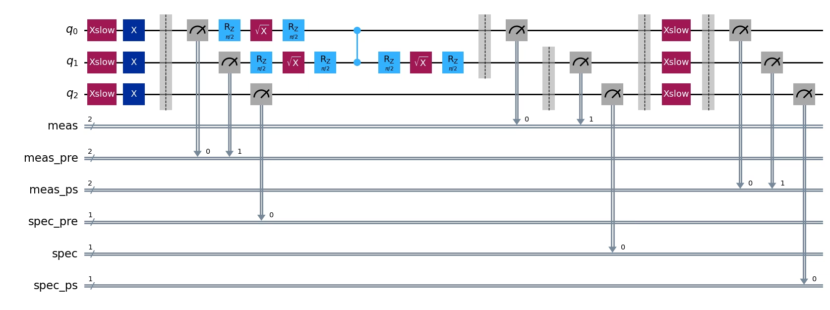
소개에서 언급했듯이, 데이터 큐비트에 인접한 보조(ancilla) 큐비트를 "관찰자(spectator)"로 사용하면 더 많은 오류를 포착할 수 있습니다. 회로 이전 및 회로 이후 관찰자 검사를 추가합니다. ibm_kingston의 물리 큐비트 2는 데이터 큐비트 1에 인접해 있으므로 관찰자로 추가되었고, 이 큐비트에 회로 이전 및 이후 검사가 추가된 것을 확인할 수 있습니다. 관찰자 측정은 spec_pre와 spec이라는 새로운 고전 레지스터에 추가되었습니다.

이와 같은 회로는 가능한 모든 비마르코프 오류 검사를 포함하므로, 이 회로에서 샘플링하면 사용자가 [회로 이전/이후] 검사와 [노드/에지] 기반 사후 선택 전략의 어떤 조합으로도 사후 선택을 할 수 있습니다. 양자 하드웨어에서 어떻게 동작하는지는 이 가이드의 2부를 참조하세요.

from qiskit_mitigation.postselection.passes import (
    AddSpectatorPostCircuitNonMarkovianErrorChecks,
    AddSpectatorPreCircuitNonMarkovianErrorChecks,
)

qc_w_checks = PassManager(
    [
        AddSpectatorPreCircuitNonMarkovianErrorChecks(
            coupling_map=backend.coupling_map
        ),
        AddSpectatorPostCircuitNonMarkovianErrorChecks(
            coupling_map=backend.coupling_map
        ),
    ]
).run(qc_w_checks)
qc_w_checks.draw("mpl", idle_wires=False, fold=-1)

2부: QPU에서 비마르코프 오류 검사를 시연하고 사후 선택 전략 비교하기

이제 비마르코프 오류 검사가 무엇이고 소프트웨어에서 어떻게 구현되는지 이해했으니, QPU에서 더 큰 예제를 실행하여 어떻게 동작하는지 확인해 볼 수 있습니다. 먼저 회로를 준비합니다. 회로의 선택은 그다지 중요하지 않으며, 출력을 쉽게 검증할 수 있는 회로이면 충분합니다. 여기서는 20 큐비트 1차원 미러링 Ising 회로를 선택합니다. 이 회로는 하드웨어에서 실행하기가 간단하지 않고 비마르코프 오류의 영향을 받을 것이므로, 비마르코프 오류 검사의 효과를 보여 줄 기회가 됩니다. 또한 미러링 구조 덕분에 노이즈가 있는 기댓값 계산을 정확한 값과 손쉽게 비교할 수 있습니다.

이 실험에서는 관측량의 기댓값을 계산합니다. 관측량 $O$의 선택도 중요하지 않으므로, 단순히 평균 단일 사이트 자화 $O=\frac{1}{N}\sum_i\langle Z_i\rangle$를 선택합니다.

import numpy as np
from qiskit.quantum_info import SparsePauliOp
from qiskit.transpiler import CouplingMap

num_qubits = 20
initial_layout = initial_layout = [
    124,
    125,
    126,
    127,
    128,
    129,
    130,
    131,
    132,
    133,
    134,
    135,
    139,
    155,
    154,
    153,
    152,
    151,
    150,
    149,
][:num_qubits]
coupling_map = CouplingMap.from_line(num_qubits, bidirectional=False)

# Num Trotter steps and `rx` angle
num_steps = 6
theta_rx = np.pi / 6

# Average single-site magnetization
observable = (
    SparsePauliOp(
        [
            "I" * iq + "Z" + "I" * (num_qubits - iq - 1)
            for iq in range(num_qubits)
        ]
    )
    / num_qubits
)

# Create the Trotter circuit
circuit = QuantumCircuit(num_qubits)
edges = CouplingMap.from_line(num_qubits, bidirectional=False).get_edges()
edges_a = [e for e in edges if e[0] % 2 == 0]
edges_b = [e for e in edges if e[0] % 2 == 1]
for _ in range(num_steps):
    circuit.rx(theta_rx, [i for i in range(num_qubits)])
    for edge in edges_a:
        circuit.cz(edge[0], edge[1])
    for edge in edges_b:
        circuit.cz(edge[0], edge[1])
circuit = circuit.compose(circuit.inverse())
circuit.measure_all()

# Transpile circuit to backend
pm = generate_preset_pass_manager(
    optimization_level=0, backend=backend, initial_layout=initial_layout
)
isa_circuit = pm.run(circuit)
print(
    f"two-qubit depth: {isa_circuit.depth(lambda instr: instr.operation.num_qubits == 2)}"
)
print(f"total depth:     {isa_circuit.depth()}")
isa_circuit.draw("mpl", fold=-1, idle_wires=False)

two-qubit depth: 24
total depth:     85

이제 인접한 관찰자 큐비트 7개를 포함하여 모든 큐비트에 회로 이전 및 이후 검사를 추가합니다. 가능한 모든 검사를 회로에 추가하면, 후처리 단계에서 어떤 사후 선택 전략을 사용할지 정할 수 있습니다.

# Use all non-Markovian error checks so we can compare all strategies in post-processing.
combined = PassManager(
    [
        AddPreCircuitNonMarkovianErrorChecks(x_pulse_type="rx"),
        AddSpectatorPreCircuitNonMarkovianErrorChecks(
            backend.coupling_map, x_pulse_type="rx"
        ),
        AddPostCircuitNonMarkovianErrorChecks(x_pulse_type="rx"),
        AddSpectatorPostCircuitNonMarkovianErrorChecks(
            backend.coupling_map, x_pulse_type="rx"
        ),
    ]
).run(isa_circuit)
combined_isa = generate_preset_pass_manager(
    optimization_level=0, backend=backend
).run(combined)

print("cregs:", [(c.name, c.size) for c in combined_isa.cregs])

cregs: [('meas', 20), ('meas_pre', 20), ('spec_pre', 7), ('meas_ps', 20), ('spec', 7), ('spec_ps', 7)]

Executor 프리미티브를 사용하여 검사가 포함된 회로를 샘플링합니다.

from qiskit_ibm_runtime import Executor
from samplomatic.quantum_program import QuantumProgram

# Raw and combined-checks circuits in a single 100k-shot program so they share calibration.
program = QuantumProgram(shots=100_000)
program.append_circuit_item(isa_circuit)  # raw circuit, no checks
program.append_circuit_item(
    combined_isa
)  # combined pre + post non-Markovian error checks
job = Executor(backend).run(program)
print(f"job id: {job.job_id()}")
print(f"status: {job.status()}")

job id: d9badrm6hjac73ffe31g
status: QUEUED

PostSelector 클래스는 검사의 creg 구조를 알고 있으므로, 샘플의 각 비트를 그에 해당하는 회로 측정과 연결할 수 있습니다. compute_mask 메서드를 사용하면 사후 선택 전략(노드 또는 에지)과 살펴볼 비마르코프 오류 검사의 유형(회로 이전 또는 이후)이 주어졌을 때 샘플 시퀀스에 대한 마스크를 만들 수 있습니다. 회로 이전 및 이후 전략을 하나의 마스크로 결합하려면 각각의 마스크를 독립적으로 계산한 다음 AND 연산으로 결합하면 됩니다. 여기서는 PostSelector를 사용해 다양한 전략의 마스크를 모두 만들고, 사용 가능한 전략의 모든 순열에 대해 결과를 살펴봅니다.

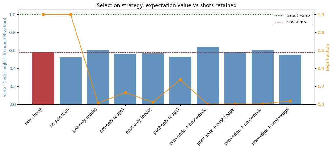
아래 시각화에서 사후 선택 전략이 사후 선택 비율과 답의 품질에 어떤 영향을 미치는지 볼 수 있습니다. 예상대로 노드 기반 사후 선택을 사용하는 전략은 사후 선택 비율이 가장 낮았습니다. 에지 기반 전략은 더 관대하여 사후 선택 비율이 더 높은 경향이 있습니다. 사용자는 문제에 맞는 다양한 전략을 시도해 보면서 사후 선택 비율과 샘플링된 분포의 품질 사이에서 적절한 균형을 찾아야 합니다. 이 예제에서는 회로 이전 및 이후 검사와 함께 노드 기반 사후 선택을 사용했을 때 사후 선택 비율 .028%로 가장 좋은 답을 얻었습니다. 일부 전략은 원본 회로보다 나은 성능을 내지 못했습니다. 또한 검사를 추가하고도 그중 어느 것도 사용하지 않은 경우(아래 차트에서 "no selection"으로 표시된 막대)가 가장 나쁜 성능을 보인다는 것도 확인할 수 있습니다.

import matplotlib.pyplot as plt
from qiskit_mitigation.postselection import PostSelector

selector = PostSelector.from_circuit(combined_isa, backend.coupling_map)

exec_results = job.result()
# The Executor returns numpy arrays keyed by classical-register name, so each result item is
# already the {creg_name: ndarray} mapping that compute_mask expects.
raw_bits = exec_results[0]["meas"]  # raw circuit, no checks
bits = exec_results[1]  # combined pre+post circuit

meas_bits = bits["meas"]
total = meas_bits[..., 0].size

def magnetization(b, mask=None):
    """Average single-site magnetization over the (optionally masked) measurement bits."""
    kept = b if mask is None else b[mask]
    return (1 - 2 * kept.astype(int)).mean()  # bit 0 -> +1, bit 1 -> -1

rows = []

def report(label, mask=None, b=meas_bits):
    """Record and print the magnetization and kept fraction for one selection strategy."""
    kept = b[..., 0].size if mask is None else int(mask.sum())
    ev = magnetization(b, mask)
    rows.append((label, ev, kept / total))
    print(f"{label:<24}: <m> = {ev:+.4f}   (kept {kept:>6}/{total})")

# Compare all possible postselection strategies
report("raw circuit", b=raw_bits)
report("no selection")
for s in ("node", "edge"):
    report(f"pre-only ({s})", selector.compute_mask(bits, s, mode="pre"))
for s in ("node", "edge"):
    report(f"post-only ({s})", selector.compute_mask(bits, s, mode="post"))
for pre_s in ("node", "edge"):
    for post_s in ("node", "edge"):
        keep = selector.compute_mask(
            bits, pre_s, mode="pre"
        ) & selector.compute_mask(bits, post_s, mode="post")
        report(f"pre={pre_s} + post={post_s}", keep)

labels = [r[0] for r in rows]
evs = [r[1] for r in rows]
fracs = [r[2] for r in rows]
x = range(len(labels))

fig, ax1 = plt.subplots(figsize=(11, 5))

# Bars: expectation value per selection strategy.
bar_colors = ["firebrick"] + ["steelblue"] * (len(evs) - 1)
ax1.bar(x, evs, color=bar_colors, alpha=0.85)
ax1.axhline(1.0, color="green", ls=":", lw=1.5, label="exact <m>")
ax1.axhline(rows[0][1], color="firebrick", ls="--", lw=1, label="raw <m>")
ax1.set_ylabel("<m>  (avg single-site magnetization)", color="steelblue")
ax1.tick_params(axis="y", labelcolor="steelblue")
ax1.set_xticks(list(x))
ax1.set_xticklabels(labels, rotation=45, ha="right")
ax1.legend(loc="upper right")

# Line: fraction of shots retained (right axis).
ax2 = ax1.twinx()
ax2.plot(x, fracs, "o-", color="darkorange")
ax2.set_ylabel("kept fraction", color="darkorange")
ax2.tick_params(axis="y", labelcolor="darkorange")
ax2.set_ylim(0, 1.05)

ax1.set_title("Selection strategy: expectation value vs shots retained")
fig.tight_layout()
plt.show()

raw circuit             : <m> = +0.5791   (kept 100000/100000)
no selection            : <m> = +0.5211   (kept 100000/100000)
pre-only (node)         : <m> = +0.6026   (kept   1357/100000)
pre-only (edge)         : <m> = +0.5637   (kept  13029/100000)
post-only (node)        : <m> = +0.5682   (kept   2254/100000)
post-only (edge)        : <m> = +0.5265   (kept  27514/100000)
pre=node + post=node    : <m> = +0.6393   (kept     28/100000)
pre=node + post=edge    : <m> = +0.5799   (kept    442/100000)
pre=edge + post=node    : <m> = +0.6006   (kept    317/100000)
pre=edge + post=edge    : <m> = +0.5521   (kept   3836/100000)