gate folding과 사용자 정의 외삽을 사용한 zero-noise 외삽
Zero-noise 외삽(ZNE)은 관측량 기댓값 계산에서 양자 노이즈를 완화하는 기법입니다. 양자 회로를 점점 커지는 노이즈 스케일에서 실행하고, 그 노이즈 스케일에 대한 기댓값을 구한 다음, 외삽하여 zero-noise 기댓값을 추정하는 방식으로 작동합니다. 노이즈 증폭 단계와 외삽 단계는 모두 다양한 방식으로 구현할 수 있습니다. 이 가이드는 "디지털 gate folding"으로 노이즈를 증폭합니다. 이는 두 큐비트 gate를 해당 gate와 그 역의 동등한 시퀀스로 대체한다는 뜻입니다. 예를 들어 유니터리 를 로 대체하면 노이즈 증폭 계수는 3이 됩니다. 확률적 오류 증폭(PEA)으로 증폭을 구현할 수도 있습니다. 이 방법은 노이즈 모델을 학습하는 추가 단계가 필요하며 확률적 오류 증폭 가이드에서 다룹니다. 이 가이드는 내장된 몇 가지 피팅 전략(선형 및 지수)으로 외삽하며, 직접 만든 사용자 정의 피팅 함수를 구현하는 방법도 보여 줍니다.
ZNE는 다른 방법보다 낮은 샘플링 비용으로 양자 노이즈를 완화하는 데 효과적일 수 있지만, 편향(bias)에 대한 한계가 없다는 점을 유념하세요.
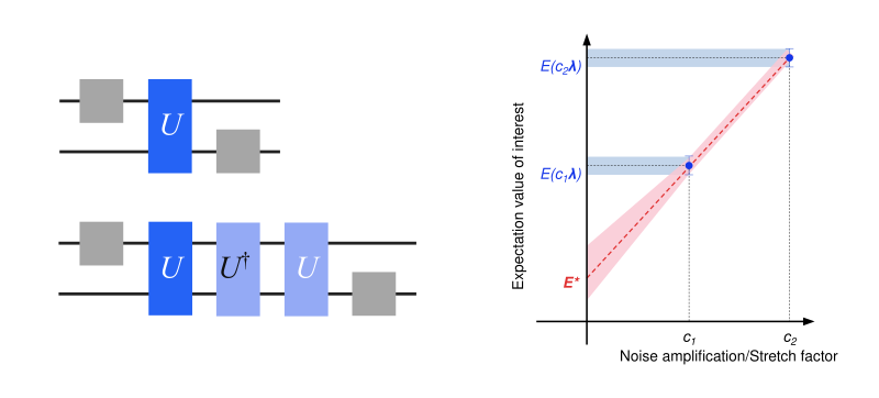
워크플로는 다음과 같습니다.
- 회로와 관측량 지정
- Qiskit의 statevector 시뮬레이터로 정확한 기댓값 계산
- 노이즈가 있는, 완화되지 않은 기댓값 계산
- 디지털 gate folding으로 ZNE 프로그램을 준비하고 노이즈 스케일이 다른 회로를 샘플링
- 내장 및 사용자 정의 피팅 함수로 zero-noise 극한까지 외삽
- 완화된 기댓값 비교
회로와 관측량 지정
링 토폴로지의 8개 큐비트에서 Trotter화된 횡자기장 Ising 모델(TFIM)의 사이트 평균 자화 를 계산합니다. 횡자기장 세기의 여러 값을 훑으면서 자화를 자기장 세기의 함수로 그립니다.
# Added by doQumentation — installs the packages this notebook needs if they are missing
import importlib.util

_needed = {"IPython": "IPython", "matplotlib": "matplotlib", "numpy": "numpy", "qiskit": "qiskit", "qiskit_aer": "qiskit-aer", "qiskit_ibm_runtime": "qiskit-ibm-runtime", "qiskit_mitigation": "qiskit-mitigation", "scipy": "scipy"}
_missing = [pip for module, pip in _needed.items()
            if importlib.util.find_spec(module) is None]
# One at a time, so a package that fails to install does not block the others
for _pip in _missing:
    %pip install -q {_pip}
if not _missing:
    print("\u2713 All required packages are installed")
import warnings

import numpy as np
from qiskit.circuit import Parameter, QuantumCircuit
from qiskit.quantum_info import SparsePauliOp

warnings.filterwarnings("ignore")

def trotter_circuit(num_qubits, theta, layers, num_steps):
    """Trotterized transverse-field Ising evolution: RX on every site, then a CZ layer per coupling layer."""
    circuit = QuantumCircuit(num_qubits)
    for _ in range(num_steps):
        circuit.rx(theta, range(num_qubits))
        for layer in layers:
            circuit.barrier()
            for edge in layer:
                circuit.cz(*edge)
                circuit.sdg(edge)
            circuit.barrier()
    return circuit

num_qubits = 8
trotter_steps = 15
ring_coupling = [(i, (i + 1) % num_qubits) for i in range(num_qubits)]
layers = [
    ring_coupling[0::2],
    ring_coupling[1::2],
]  # two disjoint layers of CZ gates
theta = Parameter("theta")
circuit = trotter_circuit(num_qubits, theta, layers, trotter_steps)

# Parameter values: theta in [0, 0.25 pi] - values for the transverse-field sweep
data_points = 6
parameter_values = np.linspace(0, 0.25 * np.pi, data_points).reshape(
    (data_points, 1)
)

# Define observables - Z on each site
observables = [
    SparsePauliOp("I" * (num_qubits - q - 1) + "Z" + "I" * q)
    for q in range(num_qubits)
]

print("Visualization of 1 Trotter step")
trotter_circuit(num_qubits, theta, layers, 1).draw("mpl", scale=0.7)
Visualization of 1 Trotter step

Qiskit의 statevector 시뮬레이터로 정확한 기댓값 계산
Qiskit의 Statevector 클래스를 사용하여 의 모든 값에 대해 각 사이트에서 의 정확한 기댓값을 계산합니다.
import matplotlib.pyplot as plt
from qiskit.quantum_info import Statevector

exact_evs = np.array(
    [
        [
            Statevector(circuit.assign_parameters([value]))
            .expectation_value(obs)
            .real
            for value in parameter_values.ravel()
        ]
        for obs in observables
    ]
)  # shape (observables, parameter values)

x_vals = parameter_values.ravel() / np.pi
fig, ax = plt.subplots(figsize=(7, 4))
ax.plot(x_vals, exact_evs.mean(axis=0), "ko-", label="Exact")
ax.set_xlabel(r"$\theta/\pi$")
ax.set_ylabel(r"$\langle Z \rangle_{\text{avg}}$")
ax.legend()
plt.tight_layout()
plt.show()

노이즈가 있는, 완화되지 않은 기댓값 계산
QuantumProgram은 Executor primitive에 적합한 형식의 양자 회로와 samplex를 담고 있습니다. MitigationTask.prepare는 회로, 관측량, 파라미터 값으로 QuantumProgram을 만들고, 주어진 boxing 옵션으로 회로를 box로 묶습니다. measure_annotations boxing 옵션을 "change_basis"로 설정하여 측정을 필요한 기저로 회전시키고, 시뮬레이터가 노이즈 모델을 회로의 box에 매핑할 수 있도록 add_tags: "unique_box"를 추가합니다. 프로그램은 기본적으로 Pauli 트위링되며, 이는 하드웨어에서 코히런트 노이즈를 완화 방법이 가정하는 Pauli 노이즈로 바꿉니다. num_randomizations는 각 회로에서 트위링된 인스턴스를 몇 개 샘플링할지 정하고 shots_per_randomization은 각 인스턴스가 몇 샷을 받을지 정하므로, 둘의 곱이 회로당 샷 예산이 됩니다.
QPU에 접근할 수 있는 사용자는 QiskitRuntimeService의 Backend로 만든 Executor로 프로그램을 실행합니다. 여기서는 Executor에 AerSimulator를 전달해 프로그램을 로컬에서 실행하고, 그 layer_noise_model 시뮬레이터 옵션을 사용하여 얽힘 gate의 모든 레이어에 무작위 Pauli-Lindblad 노이즈 모델을 주입합니다. 이 모델은 qiskit-mitigation의 random_pauli_lindblad_noise로 생성하며, 레이어드 gate당 오류(EPLG)는 현재 Heron QPU의 전형적인 값인 0.003입니다.
from qiskit.circuit import CircuitInstruction
from qiskit.quantum_info import PauliLindbladMap, pauli_basis
from qiskit_aer import AerSimulator
from qiskit_ibm_runtime import Executor
from qiskit_mitigation import MitigationTask, find_combined_unique_layers

def generate_random_pauli_lindblad_noise(
    layers,
    num_qubits: int,
    eplg: float = 3e-3,
    seed: int | None = None,
) -> list[tuple[CircuitInstruction, PauliLindbladMap]]:
    """Generate random Pauli-Lindblad noise over the full Pauli basis."""
    layer_noise_model = []
    for layer in layers:
        layer_instructions = layer.operation.params[0]
        contain_measurement = any(
            inst.name.startswith("measure") for inst in layer_instructions
        )
        if contain_measurement:  # do not add measurement noise
            layer_noise = PauliLindbladMap.identity(num_qubits)
        else:
            edges = [
                (inst.qubits[0]._index, inst.qubits[1]._index)
                for inst in layer_instructions
            ]  # extract the edges of the layer

            basis_paulis = [p for p in pauli_basis(2) if np.sum(p.x + p.z)]
            rng = np.random.default_rng(seed=seed)
            num_generators = len(basis_paulis)
            rates = rng.random(len(basis_paulis)) * eplg / num_generators

            layer_noise = PauliLindbladMap.from_sparse_list(
                [
                    (pauli.to_label(), edge, rate)
                    for pauli, rate in zip(basis_paulis, rates, strict=True)
                    for edge in edges
                ],
                num_qubits=num_qubits,
            )
        layer_noise_model.append((layer, layer_noise))
    return layer_noise_model

num_randomizations = 50
shots_per_randomization = 64

boxing_options = {
    "measure_annotations": "change_basis",
    "add_tags": "unique_box",
}

# find the unique layers to generate the layered noise for
box_layers = find_combined_unique_layers(
    [circuit], custom_boxing_options=boxing_options
)
layer_noise_model = generate_random_pauli_lindblad_noise(
    box_layers, num_qubits, seed=42
)

# a local noisy simulator in place of a QPU backend
noisy_executor = Executor(
    AerSimulator(),
    options={"simulator": {"layer_noise_model": layer_noise_model}},
)

task = MitigationTask()
program = task.prepare(
    circuit=circuit,
    observables=observables,
    parameters=parameter_values,
    num_randomizations=num_randomizations,
    shots_per_randomization=shots_per_randomization,
    custom_boxing_options=boxing_options,
)
program._semantic_role = "simulation"  # flag the program for the simulator
unmitigated_res = task.postprocess(noisy_executor.run(program).result())

fig, ax = plt.subplots(figsize=(7, 4))
ax.plot(x_vals, exact_evs.mean(axis=0), "k-", label="Exact")
ax.errorbar(
    x_vals,
    np.mean(unmitigated_res.data.evs, axis=0),
    np.mean(unmitigated_res.data.stds, axis=0),
    fmt="o-",
    label="Unmitigated",
)
ax.set_xlabel(r"$\theta/\pi$")
ax.set_ylabel(r"$\langle Z \rangle_{\text{avg}}$")
ax.legend()
plt.tight_layout()
plt.show()

디지털 gate folding으로 ZNE 프로그램을 준비하고 노이즈 스케일이 다른 회로를 샘플링
노이즈 스케일이 점점 커지는 회로를 포함하는 ZNE 프로그램을 준비합니다. 각 노이즈 계수는 회로에 포함된 얽힘 gate의 배수를 나타냅니다(노이즈 계수 3.0은 원래 회로보다 세 배 많은 얽힘 gate를 담고 있습니다). 각 노이즈 계수의 회로는 완화되지 않은 프로그램과 같은 수의 무작위화와 샷으로 트위링됩니다.
from qiskit_mitigation import GateFolding

task_gf = GateFolding()
program_zne = task_gf.prepare(
    circuit=circuit,
    observables=observables,
    parameters=parameter_values,
    num_randomizations=num_randomizations,
    shots_per_randomization=shots_per_randomization,
    custom_boxing_options=boxing_options,
    noise_factors=[1, 3, 5],  # ZNE option
)
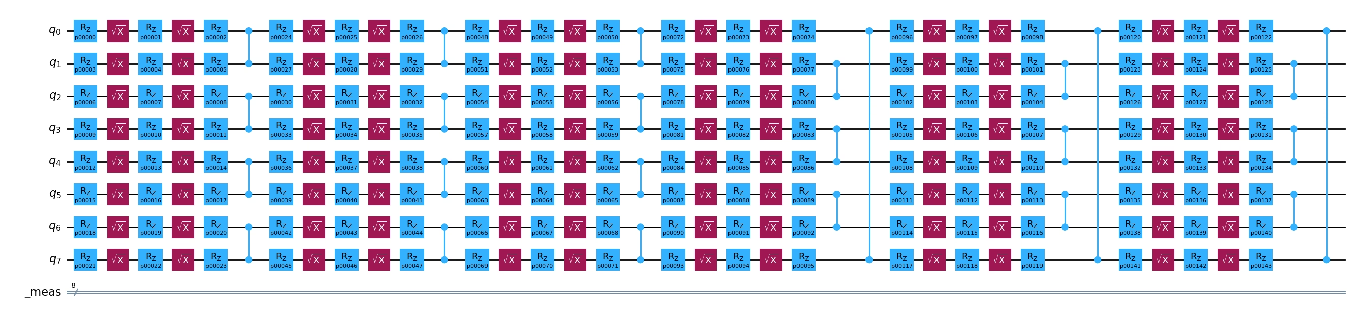
노이즈 계수 1과 노이즈 계수 3으로 트위링된 템플릿의 첫 번째 Trotter 단계를 그려서 증폭을 시각화합니다. 노이즈 계수 3.0에서는 회로의 모든 레이어가 해당 레이어, 그 역, 그리고 다시 해당 레이어로 대체됩니다.
import IPython.display

def first_trotter_step(template, noise_factor):
    """The template up to the closing barrier of its first Trotter step (two layers, each folded ``noise_factor`` times)."""
    toy = template.copy_empty_like()
    for instruction in template.data:
        toy.append(instruction)
        if (
            instruction.operation.name == "barrier"
            and instruction.operation.label.startswith(
                f"R{2 * noise_factor - 1}@"
            )
        ):
            break
    return toy

IPython.display.display(
    first_trotter_step(program_zne.items[0].circuit, 1).draw(
        "mpl", scale=0.7, plot_barriers=False
    )
)
first_trotter_step(program_zne.items[1].circuit, 3).draw(
    "mpl", fold=-1, plot_barriers=False
)

마지막으로 노이즈가 있는 시뮬레이터에서 프로그램을 실행합니다. 그 결과는 다음 단계의 외삽에 사용됩니다.
program_zne._semantic_role = (
    "simulation"  # flag the program for the simulator
)
job_zne_results = noisy_executor.run(program_zne).result()
내장 및 사용자 정의 피팅 함수로 zero-noise 극한까지 외삽
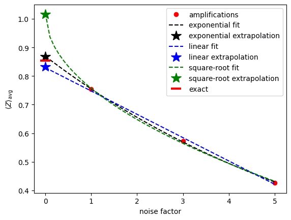
이제 각 노이즈 스케일의 데이터가 있으므로, 데이터에 함수를 피팅하고 zero-noise 값으로 되돌려 외삽하여 노이즈 없는 관측량의 기댓값을 추정할 수 있습니다. 데이터를 피팅하는 방법은 많으며, 올바른 함수 선택은 샘플링된 데이터의 성격에 따라 달라집니다. GateFolding.postprocess는 linear, exponential, double_exponential 등 여러 내장 외삽 함수를 제공합니다. postprocess 메서드는 외삽 방법의 목록을 받아 순서대로 평가하고, 물리적으로 유효한 값과 유한한 분산을 가진 첫 번째 값을 반환합니다. 즉 외삽기를 지정하는 순서가 어떤 외삽기가 선택되는지에 큰 영향을 줍니다. 외삽기로 fallback을 제출하면 유효한 답을 찾지 못한 경우 가장 작은 노이즈 계수의 기댓값이 선택되어 반환됩니다. fallback을 제출하지 않았고 어떤 외삽기도 물리적으로 유효한 값을 내지 못하면, std가 가장 작은 결과가 반환됩니다. Pauli 노이즈에서는 관측량이 노이즈 계수에 따라 지수적으로 감쇠하므로, 얽힘 gate의 30개 레이어(15개 Trotter 단계, 단계당 2개 레이어)에서는 지수 외삽기가 자연스러운 선택입니다. 감쇠가 작을 때 흔히 쓰이는 선형 외삽도 할 수 있습니다.
사용자 정의 피팅 함수를 사용하려면 "custom" 외삽기를 피팅 함수, 각 파라미터의 초기 추정값 목록, 그리고 경계를 담은 custom_fit 튜플과 함께 전달하세요. 이 값들은 scipy.optimize.curve_fit로 전달됩니다. 후처리는 프로그램을 다시 실행하지 않고도 다른 외삽기로 반복할 수 있습니다. 여기서는 사용자 정의 제곱근 피팅 함수를 사용합니다. 외삽을 시각화하기 위해, 에서 각 노이즈 계수마다 계산한 사이트 평균 자화, 세 가지 피팅, 그리고 zero-noise 지점에서 외삽된 기댓값의 사이트 평균을 그립니다. 세 데이터 점은 거의 선형으로 보이지만, 선형 외삽은 정확한 값보다 눈에 띄게 아래에 놓입니다. 예측대로 지数 피팅이 노이즈 없는 기댓값을 가장 효과적으로 추정합니다.
from scipy.optimize import curve_fit

zne_mitigated_exp = task_gf.postprocess(
    job_zne_results, extrapolator=["exponential", "linear"]
)
zne_mitigated_lin = task_gf.postprocess(
    job_zne_results, extrapolator=["linear"]
)

def sqrt_fit(x, a, b):
    return a * np.sqrt(x) + b

custom_fit = (sqrt_fit, [1.0, 1.0], (-np.inf, np.inf))
zne_mitigated_custom = task_gf.postprocess(
    job_zne_results,
    extrapolator=["custom", "exponential", "linear"],
    custom_fit=custom_fit,
)

# The result holds the expectation value at each noise factor and the extrapolated value, but
# not the fit parameters, so we refit the same models here to draw the curves.
noise_factors = np.array([1, 3, 5])
angle = 3  # theta = 0.15 pi, the angle with the largest unmitigated error
amplifications = zne_mitigated_exp.data.evs_noise_factors[:, angle, :].mean(
    axis=0
)
x_fit = np.linspace(0, 5, 51)
fits = {
    "exponential": (
        lambda x, a, b: a * np.exp(b * x),
        zne_mitigated_exp,
        "black",
    ),
    "linear": (lambda x, a, b: a * x + b, zne_mitigated_lin, "blue"),
    "square-root": (sqrt_fit, zne_mitigated_custom, "green"),
}

plt.plot(
    noise_factors, amplifications, "o", color="red", label="amplifications"
)
for name, (fit, res, color) in fits.items():
    params, _ = curve_fit(fit, noise_factors, amplifications, p0=[1.0, -0.1])
    plt.plot(
        x_fit, fit(x_fit, *params), "--", color=color, label=f"{name} fit"
    )
    plt.plot(
        [0],
        res.data.evs[:, angle].mean(),
        "*",
        color=color,
        markersize=15,
        label=f"{name} extrapolation",
    )
plt.plot(
    [0],
    exact_evs[:, angle].mean(),
    "_",
    color="red",
    markersize=15,
    markeredgewidth=3,
    label="exact",
)
plt.xlabel("noise factor")
plt.ylabel(r"$\langle Z \rangle_{\text{avg}}$")
plt.legend()
plt.show()
완화된 기댓값 비교
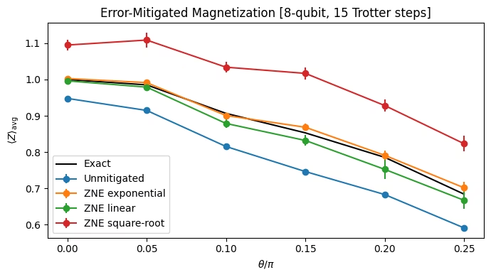
Ising 회전각에 걸친 스윕에서 각 방법의 사이트 평균 자화를 그립니다. 지수 외삽은 오차 막대 안에서 정확한 자화를 복원하는 반면, 선형 외삽은 편향을 상당 부분 제거하지만 실제 감쇠가 지수적이기 때문에 일관되게 과소 추정합니다. 제곱근 피팅은 심하게 과대 추정합니다.
results = {
    "Unmitigated": unmitigated_res,
    "ZNE exponential": zne_mitigated_exp,
    "ZNE linear": zne_mitigated_lin,
    "ZNE square-root": zne_mitigated_custom,
}

fig, ax = plt.subplots(figsize=(7, 4))
ax.plot(x_vals, exact_evs.mean(axis=0), "k-", label="Exact")
for label, res in results.items():
    ax.errorbar(
        x_vals,
        np.mean(res.data.evs, axis=0),
        np.mean(res.data.stds, axis=0),
        fmt="o-",
        label=label,
    )
ax.set_xlabel(r"$\theta/\pi$")
ax.set_ylabel(r"$\langle Z \rangle_{\text{avg}}$")
ax.legend()
ax.set_title(
    f"Error-Mitigated Magnetization [{num_qubits}-qubit, {trotter_steps} Trotter steps]"
)
plt.tight_layout()
plt.show()