SLC를 사용한 PEC

확률적 오류 상쇄(PEC)는 관측량 기댓값 계산에서 양자 노이즈를 완화하는 기법입니다. 이를 통해 기댓값의 편향 없는 추정치를 계산할 수 있습니다. 이 기법은 학습된 노이즈 모델의 역을 주입한 노이즈 Circuit들의 앙상블을 실행하는 방식으로 동작합니다. 이후 Pauli twirling(randomized compiling이라고도 함)을 사용해 노이즈 모델을 Pauli 채널로 근사합니다. 이러한 노이즈 모델은 효율적으로 학습할 수 있으며 PEC를 사용해 완화할 수 있습니다(자세한 내용은 Probabilistic error cancellation with sparse Pauli-Lindblad models on noisy quantum processors 참조).

PEC는 편향 없는 추정치를 계산하기 위해 shot 오버헤드가 지수적으로 필요합니다. Shaded Lightcones(SLC)는 고전 자원을 사용해 Circuit 전체에서 오류에 대한 민감도의 한계를 정하는 기법입니다. 이 한계를 이용해 사용자는 관측량 추정의 편향을 제어하며 조절할 수 있습니다.

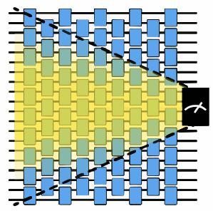
이 가이드는 PEC와 SLC를 함께 사용하여 기본 PEC보다 줄어든 shot 오버헤드로 Gate 노이즈를 완화하는 방법을 보여줍니다.

워크플로는 다음과 같습니다.

1. Circuit과 관측량을 지정합니다.
2. 노이즈가 있고 완화되지 않은 기댓값을 계산합니다.
3. 편향에 대한 순방향 및 역방향 한계를 계산합니다.
4. qiskit-noise-learning을 사용해 얽힘 레이어의 노이즈를 학습합니다.
5. 학습된 노이즈를 사용해 계산된 한계를 로컬 스케일 행렬로 병합합니다.
6. shot 오버헤드와 편향 간의 절충에 따라 원하는 편향 한계를 선택합니다.
7. PEC + SLC 프로그램을 준비하고, 프로그램을 실행한 뒤 후처리합니다.
8. 완화된 기댓값과 shot 오버헤드를 비교합니다.

Circuit과 관측량 지정하기

Qubit 8개에서 1차원 Ising 사슬 해밀토니안의 Trotter화된 시간 발전에 대한 미러 Circuit을 준비합니다. Circuit을 미러링하면 유니터리가 상쇄되어 항등 Circuit이 만들어지므로, 각 관측량의 이상적인 기댓값을 계산하지 않아도 1임을 알 수 있습니다. 또한 미러링은 Circuit 깊이를 두 배로 늘리고, 그에 따라 노이즈의 영향도 두 배가 됩니다.

각도 $\theta= \frac{\pi}{4}$를 사용해 동역학을 비Clifford로 만듭니다.

# Added by doQumentation — installs the packages this notebook needs if they are missing
import importlib.util

_needed = {"matplotlib": "matplotlib", "numpy": "numpy", "qiskit": "qiskit", "qiskit_addon_slc": "qiskit-addon-slc", "qiskit_aer": "qiskit-aer", "qiskit_ibm_runtime": "qiskit-ibm-runtime", "qiskit_mitigation": "qiskit-mitigation", "qiskit_noise_learning": "qiskit-noise-learning", "samplomatic": "samplomatic"}
_missing = [pip for module, pip in _needed.items()
            if importlib.util.find_spec(module) is None]
# One at a time, so a package that fails to install does not block the others
for _pip in _missing:
    %pip install -q {_pip}
if not _missing:
    print("\u2713 All required packages are installed")

import warnings

import numpy as np
from qiskit.circuit import QuantumCircuit
from qiskit.quantum_info import SparsePauliOp
from qiskit_mitigation.utils import get_measurement_bases

warnings.filterwarnings("ignore")

def construct_ising_circuit(
    num_qubits: int,
    num_trotter_steps: int,
    rx_angle: float,
) -> QuantumCircuit:
    circuit = QuantumCircuit(num_qubits)

    for _ in range(num_trotter_steps):
        circuit.rx(rx_angle, range(num_qubits))
        for first_qubit in (1, 2):
            for idx in range(first_qubit, num_qubits, 2):
                # equivalent to Rzz(-pi/2):
                circuit.sdg([idx - 1, idx])
                circuit.cz(idx - 1, idx)

    return circuit

def prepare_basis(
    circuit: QuantumCircuit, basis: list[int]
) -> QuantumCircuit:
    # basis is a list of integer values from 0 to 3. These map to the basis measurement as:
    # 0 = I; 1 = Z; 2 = X; 3 = Y
    assert len(basis) == circuit.num_qubits

    out_circ = circuit.copy_empty_like()
    for qb, bas in enumerate(basis):
        if bas == 2:
            out_circ.h(qb)
        elif bas == 3:
            out_circ.rx(-np.pi / 2, qb)

    out_circ.barrier()
    out_circ.compose(circuit, inplace=True)
    return out_circ

def mirror_circuit(circuit: QuantumCircuit) -> QuantumCircuit:
    mirror_circ = circuit.copy_empty_like()
    mirror_circ.compose(circuit.inverse(), inplace=True)
    mirror_circ.barrier()
    mirror_circ.compose(circuit, inplace=True)
    mirror_circ.measure_active()
    return mirror_circ

# define observables
num_qubits = 8  # Width of the Ising chain
# The observable to measure: one X component (on qubit 2) and one Z component (on qubit 5)
target_obs_sparse = [("XZ", [2, 5], 1.0)]
observable = SparsePauliOp.from_sparse_list(
    target_obs_sparse, num_qubits=num_qubits
)

# Determine the measurement basis each qubit requires for this observable.
bases, _ = get_measurement_bases(observable)

# Instantiate the mirrored circuit and prepend the basis-preparation gates
num_trotter_steps = 6
rx_angle = np.pi / 4
circuit = construct_ising_circuit(num_qubits, num_trotter_steps, rx_angle)
mirrored_circuit = mirror_circuit(circuit)
mirrored_circuit = prepare_basis(mirrored_circuit, bases[0])
print("Visualization of 1 mirrored Trotter step")
prepare_basis(
    mirror_circuit(construct_ising_circuit(num_qubits, 1, rx_angle)), bases[0]
).draw("mpl", scale=0.6, fold=-1)

Visualization of 1 mirrored Trotter step

노이즈가 있고 완화되지 않은 기댓값 계산하기

QuantumProgram은 Executor primitive에 적합한 형식으로 양자 Circuit과 samplex를 담고 있습니다. MitigationTask.prepare는 Circuit, 관측량, 매개변수 값으로 QuantumProgram을 만들고, 주어진 박싱 옵션으로 Circuit을 박스로 묶습니다. measure_annotations 박싱 옵션을 "change_basis"로 설정하면 측정이 필요한 기저로 회전되며, 시뮬레이터가 노이즈 모델을 Circuit의 박스에 매핑할 수 있도록 add_tags: "unique_box"를 추가합니다. 프로그램은 기본적으로 Pauli twirling되며, 하드웨어에서는 이것이 결맞음 노이즈를 완화 방법이 가정하는 Pauli 노이즈로 바꿉니다. num_randomizations는 각 Circuit에서 twirling된 인스턴스를 몇 개 샘플링할지 정하고, shots_per_randomization은 각 인스턴스가 받는 shot 수를 정하므로, 둘의 곱이 Circuit당 shot 한도가 됩니다.

QPU에 접근할 수 있다면 QiskitRuntimeService의 Backend로 만든 Executor로 프로그램을 실행할 수 있습니다. 이 예제에서는 AerSimulator를 사용해 프로그램을 로컬에서 실행합니다. 시뮬레이터 옵션 layer_noise_model은 주어진 Pauli-Lindblad 노이즈 모델의 노이즈를 모든 얽힘 Gate 레이어에 주입합니다. 여기서는 작은 규모의 문제에서도 SLC 사용의 효과를 크게 보여주기 위해, 레이어드 Gate당 오류(EPLG)가 현재의 일반적인 Heron QPU보다 거의 한 자릿수 높은 0.01인 무작위 Pauli-Lindblad 노이즈 모델을 생성합니다.

from qiskit.circuit import CircuitInstruction
from qiskit.quantum_info import PauliLindbladMap, pauli_basis
from qiskit_aer import AerSimulator
from qiskit_ibm_runtime import Executor
from qiskit_mitigation import MitigationTask, find_combined_unique_layers
from samplomatic import Tag
from samplomatic.utils import get_annotation

def generate_random_pauli_lindblad_noise(
    layers,
    num_qubits: int,
    eplg: float = 3e-3,
    seed: int | None = None,
) -> list[tuple[CircuitInstruction, PauliLindbladMap]]:
    """Generate random Pauli-Lindblad noise over the full Pauli basis."""
    layer_noise_model = []
    for layer in layers:
        layer_instructions = layer.operation.params[0]
        contain_measurement = any(
            inst.name.startswith("measure") for inst in layer_instructions
        )
        if contain_measurement:  # do not add measurement noise
            layer_noise = PauliLindbladMap.identity(num_qubits)
        else:
            edges = [
                (inst.qubits[0]._index, inst.qubits[1]._index)
                for inst in layer_instructions
            ]  # extract the edges of the layer

            basis_paulis = [p for p in pauli_basis(2) if np.sum(p.x + p.z)]
            rng = np.random.default_rng(seed=seed)
            num_generators = len(basis_paulis)
            rates = rng.random(len(basis_paulis)) * eplg / num_generators

            layer_noise = PauliLindbladMap.from_sparse_list(
                [
                    (pauli.to_label(), edge, rate)
                    for pauli, rate in zip(basis_paulis, rates, strict=True)
                    for edge in edges
                ],
                num_qubits=num_qubits,
            )
        layer_noise_model.append((layer, layer_noise))
    return layer_noise_model

num_randomizations = 400
shots_per_randomization = 16

boxing_options = {"add_tags": "unique_box"}

# find the unique layers to generate the layered noise for
box_layers = find_combined_unique_layers(
    [mirrored_circuit], custom_boxing_options=boxing_options
)
layer_noise_model = generate_random_pauli_lindblad_noise(
    box_layers, num_qubits, eplg=1e-2, seed=42
)

# a local noisy simulator in place of a QPU backend
noisy_executor = Executor(
    AerSimulator(),
    options={"simulator": {"layer_noise_model": layer_noise_model}},
)

task = MitigationTask()
program = task.prepare(
    circuit=mirrored_circuit,
    observables=observable,
    parameters=None,
    num_randomizations=num_randomizations,
    shots_per_randomization=shots_per_randomization,
    custom_boxing_options=boxing_options,
)

program._semantic_role = "simulation"  # flag the program for the simulator
job_unmit_res = noisy_executor.run(program).result()
unmitigated_res = task.postprocess(job_unmit_res)

print(f"unmitigated result: {unmitigated_res.data.evs[0]}")

unmitigated result: 0.63125

편향에 대한 순방향 및 역방향 한계 계산하기

노이즈 학습에 QPU 시간을 쓰기 전에, SLC는 고전 시뮬레이션을 사용해 각 잠재적 오류가 관측량의 편향에 기여하는 정도의 한계를 정합니다. 이는 서로 보완적인 두 단계로 이루어집니다.

• 순방향 전파: 각 Pauli 오류를 Circuit의 나머지 부분을 따라 순방향으로 전파하고 관측량과의 교환자를 평가합니다. 관측량과 반교환하는 오류만이 결과를 편향시킬 수 있으므로, 이 단계는 각 오류의 순방향 영향에 대한 상한을 만들어냅니다.

• 역방향 전파: 각 오류를 Circuit의 시작점까지 역방향으로 전파하고 초기 상태와의 교환자를 평가합니다. Circuit이 전부 0인 상태에서 시작하므로 이 상태와 교환하는 오류는 결과에 영향을 줄 수 없으며, 이는 반대 방향에서 한계를 더 조입니다.

두 한계를 합치면 각 오류가 편향에 미치는 최악의 기여에 대한 촘촘한 범위가 형성됩니다. 다음 단계에서는 이 한계를 학습된 노이즈 비율과 병합하여 어떤 오류를 보정할 가치가 있고 어떤 오류를 그대로 두어도 안전한지 순위를 매깁니다. 박스로 묶인 Circuit의 각 InjectNoise 주석이 SLC 한계를 연결할 수 있는 고유한 식별자를 가지려면 여기서 inject_noise_strategy="individual_modification" 박싱 옵션이 필요합니다.

더 큰 규모의 문제에서는 이러한 계산에 상당한 고전 계산 자원이 필요할 수 있습니다.

from qiskit_addon_slc.bounds import (
    compute_backward_bounds,
    compute_forward_bounds,
    tighten_with_speed_limit,
)
from qiskit_mitigation import PEC

slc_boxing_options = {
    "add_tags": "unique_box",
    "inject_noise_strategy": "individual_modification",
}

slc_pec_task = PEC()

boxed_circuit, noise_model_paulis = (
    slc_pec_task.generate_slc_bounds_computation_input(
        mirrored_circuit, custom_boxing_options=slc_boxing_options
    )
)

forward_bounds = compute_forward_bounds(
    boxed_circuit, noise_model_paulis, observable
)
tighten_forward_bounds = tighten_with_speed_limit(
    forward_bounds, boxed_circuit, noise_model_paulis, observable
)
backward_bounds = compute_backward_bounds(boxed_circuit, noise_model_paulis)

얽힘 레이어의 노이즈 학습하기

각 오류가 기댓값의 편향에 얼마나 영향을 주는지, 그리고 이를 보정하는 데 비용이 얼마나 드는지 최종적으로 추정하기 위해, 노이즈 비율을 학습하고 이를 앞서 계산한 예측 노이즈 한계에 적용합니다.

PEC(그리고 PEC+SLC)는 Circuit의 각 얽힘 Gate 레이어에 대해 twirling된 노이즈 모델을 가정합니다. 마르코프 노이즈 모델을 가정하면 Circuit의 깊이는 특정 얽힘 레이어의 노이즈 채널에 영향을 주지 않는다고 봅니다. 따라서 고유한 얽힘 Gate 레이어마다 노이즈 모델만 학습하면 됩니다. 이 가이드에서 사용하는 Circuit은 두 개의 고유한 레이어로 나눌 수 있습니다. 노이즈 모델을 학습하려는 경우, 고유한 레이어는 독립적으로 학습해야 하므로 고유한 얽힘 레이어의 집합이 최소가 되도록 Circuit을 설계하는 것이 중요합니다. Circuit에 고유한 레이어가 너무 많으면 많은 레이어를 학습하는 샘플링 비용 때문에 노이즈 학습이 불가능해질 수 있습니다.

노이즈 학습에는 qiskit-noise-learning을 사용합니다. 학습기는 학습용 Circuit에서 각 레이어를 _fragment_depths_번 반복하고, 각 Circuit을 _num_randomizations_번 twirling하며, 측정된 충실도의 감쇠를 Pauli-Lindblad 모델에 맞춥니다. 이 매개변수들은 학습된 모델의 정확도에 영향을 줄 수 있습니다. 학습된 노이즈 모델이 정확할수록 노이즈 상쇄도 더 정확해집니다.

다음 코드는 두 레이어를 하나의 맵으로 합쳐 학습된 노이즈 모델을 그립니다. 각 Qubit은 두 레이어에 걸쳐 합산한 가중치 1의 X, Y, Z 비율을 파이 차트로 나타내고, 각 엣지는 학습된 가중치 2의 비율을 보여줍니다. 예를 들어 3e-4라는 비율은 레이어를 10,000번 사용할 때 해당 오류가 대략 세 번 발생한다는 뜻입니다.

from qiskit.providers.fake_provider import GenericBackendV2
from qiskit.quantum_info import PauliList
from qiskit_ibm_runtime.results import LayerError, PauliLindbladError
from qiskit_ibm_runtime.visualization.embeddings import Embedding
from qiskit_noise_learning.aer_executor import AerExecutor
from qiskit_noise_learning.noise_learner import LearningOptions, NoiseLearner
from samplomatic import InjectNoise

line_coupling = [(i, i + 1) for i in range(num_qubits - 1)]
backend = GenericBackendV2(
    num_qubits=num_qubits,
    basis_gates=["id", "rz", "sx", "x", "cz"],
    coupling_map=line_coupling,
)

# first learn only the layers PEC will inject noise into, i.e. not the measurement layer
pec_layers = [
    layer
    for layer in slc_pec_task.find_unique_layers(
        mirrored_circuit, slc_boxing_options
    )
    if get_annotation(layer.operation, InjectNoise)
]
layers = slc_pec_task.find_unique_layers(mirrored_circuit, slc_boxing_options)

learning_options = LearningOptions(
    fragment_depths=[2, 4, 8, 16],
    num_randomizations=250,
    shots_per_randomizations=16,
)

# qiskit-noise-learning is not compatible with the Executor in local mode,
# and requires the simulator present in the package for running simulation
noise_dict = {
    get_annotation(layer.operation, Tag).ref: noise_layer
    for layer, noise_layer in layer_noise_model
}
noise_learner_simulator = AerExecutor(
    qasm_simulator=AerSimulator(), noise_dict=noise_dict
)
learner = NoiseLearner(
    backend, options=learning_options, executor=noise_learner_simulator
)
learned_noise = (
    learner.run(pec_layers).result().to_dict()
)  # keyed by InjectNoise reference

# Draw the learned model on the line, laid out as a line with the qubits in order.
# Composing the two layers' maps sums their rates, giving one map over all the edges.
embedding = Embedding(
    [(0, 0), (0, 2), (0, 4), (2, 4), (4, 4), (4, 2), (4, 0), (2, 0)],
    line_coupling,
)
first, second = learned_noise.values()
learned_model = first.compose(second).simplify()
error = PauliLindbladError(
    PauliList(
        learned_model.get_qubit_sparse_pauli_list_copy().to_pauli_list()
    ),
    learned_model.rates,
)
fig = LayerError(circuit, list(range(num_qubits)), error).draw_map(
    embedding, radius=0.4, height=460, width=620
)
fig.update_traces(
    marker={
        "cmin": 0,
        "cmax": max(learned_model.rates),
        "colorbar": {"tickformat": ".1e", "title": "rate"},
    },
    selector={"mode": "markers"},
)
fig.show()

학습된 노이즈를 사용해 계산된 한계를 로컬 스케일 행렬로 병합하기

이전 단계의 고전 한계와 학습된 노이즈 비율을 모두 확보했으므로, 이제 로컬 스케일 행렬을 계산할 수 있습니다. 이는 PEC가 각 개별 노이즈 항을 얼마나 적극적으로 상쇄할지를 결정하는 오류별 가중치입니다.

SLC의 핵심 아이디어는 모든 오류를 완전히 상쇄할 필요는 없다는 것입니다. 순방향 한계와 역방향 한계가 모두 작은 오류는 비율과 상관없이 관측량에 미치는 영향이 무시할 만하므로, 부분적으로 또는 완전히 완화하지 않고 둘 수 있습니다. merge_bounds는 고전 한계를 학습된 Pauli-Lindblad 비율과 병합하고, 그다음 compute_local_scales가 사용자가 지정한 bias_tolerance에 따라 각 오류에 0(완전히 무시)에서 1(완전히 상쇄) 사이의 스케일을 할당합니다. 편향 기여가 크다고 추정되는 오류는 1에 가까운 스케일(완전한 PEC 처리)을 받고, 기여가 작은 오류는 더 낮은 스케일을 받아 그들이 지니는 샘플링 오버헤드가 줄어듭니다.

SLC는 두 극단, 즉 기본 PEC(편향 0, 가장 높은 오버헤드)와 완화 없음(오버헤드 0, 노이즈 편향 전체) 사이에서 연속적인 조절 수단을 제공합니다. bias_tolerance 매개변수가 이를 조절합니다. 0으로 설정하면 완전한 PEC가 되고, 값이 클수록 잔여 편향을 더 허용하는 대신 샘플링 오버헤드 γ²이 낮아집니다.

이 단계에서는 bias_tolerance를 여러 값에 걸쳐 변화시키며 각 값에 대한 샘플링 오버헤드를 계산합니다. 이 지점들을 완전한 PEC의 오버헤드와 비교해 그려 보면 shot 예산에 맞는 작동점을 고르는 데 도움이 됩니다. 예를 들어 5 %의 잔여 편향을 허용하면 완전한 PEC에 비해 샘플링 오버헤드가 한 자릿수만큼 줄어들 수 있어, 그렇지 않았다면 불가능했을 계산을 오늘날의 QPU에서 수행할 수 있게 됩니다.

import matplotlib.pyplot as plt
from qiskit_addon_slc.bounds import compute_local_scales, merge_bounds

merged_bounds = merge_bounds(
    boxed_circuit,
    tighten_forward_bounds,
    backward_bounds,
    noise_rates=learned_noise,
)

biases = []
costs = []
for bias in [0.0, *np.arange(0.01, 0.11, 0.01).tolist()]:
    _, cost_, bias_ = compute_local_scales(
        boxed_circuit,
        merged_bounds,
        noise_rates=learned_noise,
        bias_tolerance=bias,
    )
    biases.append(bias_)
    costs.append(cost_)

# Compute tha full PEC overhead and compare it with the overhead and bias of different SLC configurations
vanilla_gamma = slc_pec_task.calculate_gamma(
    slc_pec_task.boxed_circuit, learned_noise, 1
)

xticks = np.arange(0, 11, 2)

fig, ax = plt.subplots()
ax.scatter(
    [0], [vanilla_gamma**2], marker="D", c="tab:orange", label="full PEC"
)
ax.plot(
    100 * np.array(biases),
    np.array(costs),
    "o-",
    c="tab:blue",
    label="PEC+SLC",
)
ax.set_xticks(xticks, [f"{x:.2f}" for x in xticks])

ax.set_xlabel("Remaining bias [%]")
ax.set_ylabel(r"Sampling overhead, $\gamma^2$")
ax.grid()
ax.legend()
fig.suptitle("PEC sampling overhead reduction due to SLC")

Optimal spacetime partitioning not implemented! Just partitioning list of noisy boxes.

Text(0.5, 0.98, 'PEC sampling overhead reduction due to SLC')

shot 오버헤드와 편향 간의 절충에 따라 원하는 편향 한계 선택하기

이 가이드에서는 편향 허용치를 5%로 선택합니다. 이 편향 계산은 학습된 노이즈 모델을 기반으로 하며, 이는 장치의 실제 노이즈와 완벽하게 일치하지 않을 수 있다는 점에 유의하세요.

chosen_bias_threshold = 0.05
local_scales, sampling_cost, bias = compute_local_scales(
    boxed_circuit, merged_bounds, learned_noise, bias_tolerance=bias
)
slc_pec_task.set_slc_local_scales(
    local_scales, float(np.sqrt(sampling_cost)), bias
)

PEC + SLC 프로그램을 준비하고, 프로그램을 실행한 뒤 후처리하기

로컬 스케일을 선택했으므로 이제 전체 PEC+SLC 실행 프로그램을 만들 수 있습니다. PEC.prepare 호출은 Circuit의 박스 주석에 반노이즈 주입 전략을 인코딩한 QuantumProgram을 구성합니다. noise_gain="slc_local_scales"를 전달하면 기본 PEC처럼 모든 오류에 동일한 전체 역노이즈 이득을 적용하는 대신, set_slc_local_scales로 설정한 오류별 가중치를 executor가 사용하도록 지시합니다.

공정한 비교를 위해 noise_gain=0인 두 번째 PEC 작업을 준비합니다. 이는 SLC 편향 허용치가 없는 완전한 PEC 상쇄에 해당합니다. 두 프로그램은 같은 QuantumProgram에 추가되어 하나의 실행 job을 공유하므로, 두 프로그램의 Circuit이 번갈아 배치되어 함께 실행되며, 따라서 하드웨어 드리프트가 둘 모두에 똑같이 영향을 줍니다.

job이 완료된 후 postprocess는 각 작업에 알맞은 PEC 재조정 인자 γ를 적용하여 원시 측정 비트열을 기댓값으로 변환합니다.

program_pec = slc_pec_task.prepare(
    circuit=mirrored_circuit,
    observables=[observable],
    parameters=None,
    num_randomizations=num_randomizations,
    shots_per_randomization=shots_per_randomization,
    custom_boxing_options=slc_boxing_options,
    noise_maps=learned_noise,  # PEC option
    noise_gain="slc_local_scales",  # PEC option. Defines the usage of SLC
    max_sampling_overhead=100,  # PEC option
)

full_pec_task = PEC()
program_pec = full_pec_task.prepare(
    circuit=mirrored_circuit,
    observables=[observable],
    parameters=None,
    num_randomizations=num_randomizations,
    shots_per_randomization=shots_per_randomization,
    custom_boxing_options=boxing_options,
    quantum_program=program_pec,
    noise_maps=learned_noise,  # PEC option
    noise_gain=0,  # PEC option
    max_sampling_overhead=100,  # PEC option
)

# Execute
program_pec._semantic_role = (
    "simulation"  # flag the program for the simulator
)
job_pec_results = noisy_executor.run(program_pec).result()

# post-processing
pec_slc_res = slc_pec_task.postprocess(job_pec_results)
full_pec_res = full_pec_task.postprocess(job_pec_results)

완화된 기댓값과 shot 오버헤드 비교하기

미러 Circuit의 이상적인 기댓값은 구성상 1이므로, 어떤 추정치의 편향이든 단순히 |1 - result|입니다. 이 마지막 셀은 세 가지 시나리오의 편향과 전체 shot 수를 나란히 출력합니다.

• 완화 없음: 오류 상쇄를 적용하지 않은 원시 노이즈 기댓값입니다.

• 완전한 PEC: 모든 레이어에서 전체 역노이즈 모델을 사용하는 편향 0의 오류 상쇄이며, 전체 γ² 샘플링 오버헤드가 듭니다.

• PEC+SLC: shaded-lightcone 로컬 스케일의 안내를 받는 오류 상쇄로, 선택한 bias_tolerance를 허용하는 대신 shot 수가 크게 줄어듭니다.

세 행을 비교하면 SLC의 구체적인 이점을 알 수 있습니다. PEC+SLC의 완화된 편향은 완화되지 않은 편향보다 훨씬 낮게 유지되면서, 전체 shot 수는 완전한 PEC에 필요했던 것보다 크게 적습니다.

print(
    f"Unmitigated result bias: {np.abs(1 - unmitigated_res.data.evs[0]) * 100:.2f}%, \
total shots ran: {job_unmit_res[0]['_meas'].shape[0] * job_unmit_res[0]['_meas'].shape[2]}"
)

print(
    f"Full PEC final result bias: {np.abs(1 - full_pec_res.data.evs[0]) * 100:.2f}%, \
total shots ran: {job_pec_results[1]['_meas'].shape[0] * job_pec_results[1]['_meas'].shape[2]}"
)

print(
    f"PEC+SLC final result bias: {np.abs(1 - pec_slc_res.data.evs[0]) * 100:.2f}%, \
total shots ran: {job_pec_results[0]['_meas'].shape[0] * job_pec_results[0]['_meas'].shape[2]}"
)

Unmitigated result bias: 36.88%, total shots ran: 6400
Full PEC final result bias: 0.97%, total shots ran: 48528
PEC+SLC final result bias: 1.46%, total shots ran: 24480