논리 노이즈 모델을 사용한 확률적 오류 상쇄
사용량 추정치: Heron r3 프로세서에서 28분 (참고: 이는 추정치일 뿐입니다. 실제 실행 시간은 다를 수 있습니다.)
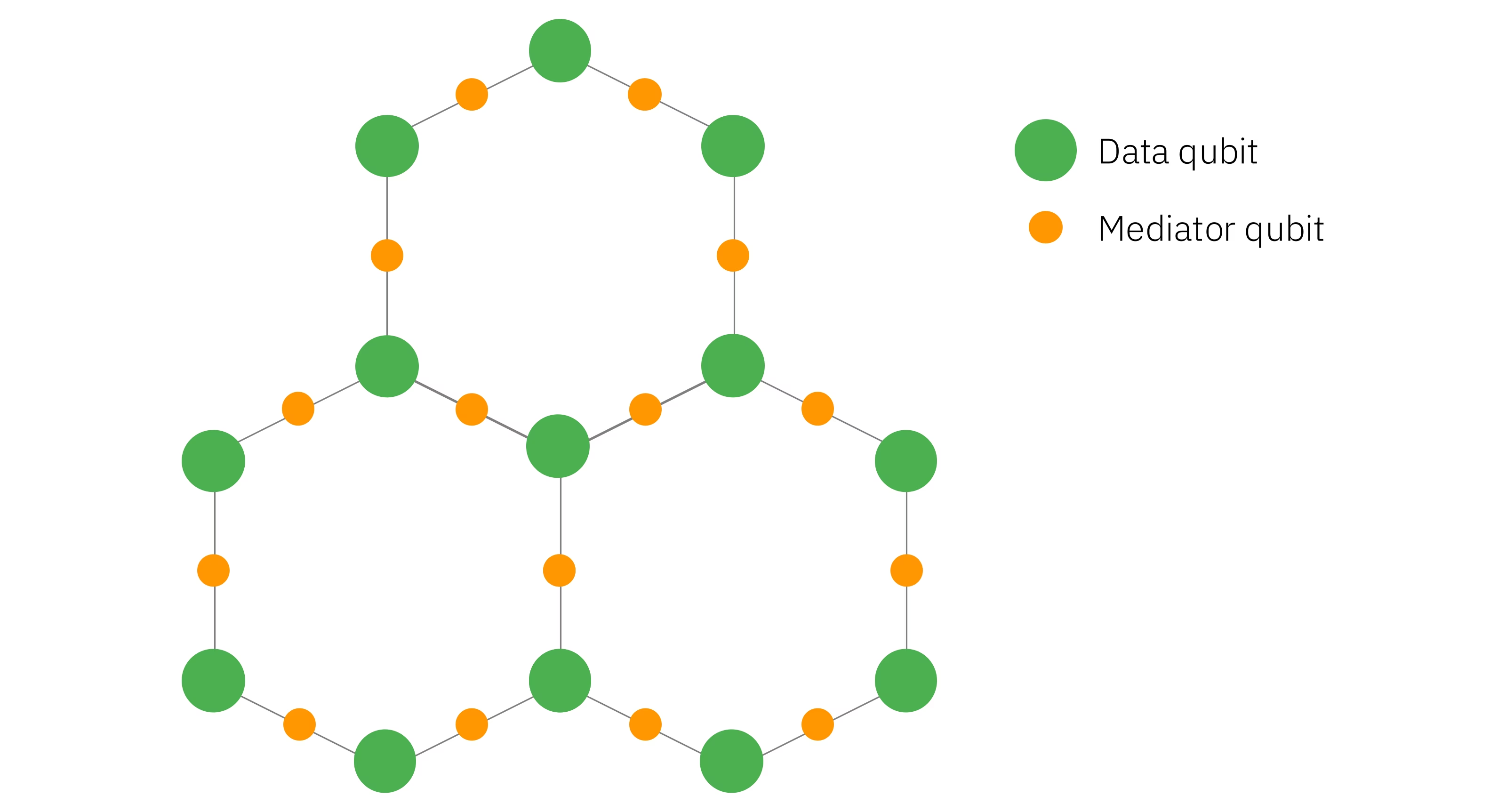 In this tutorial we will evaluate observables of a 22-site Ising model on a hexagonal lattice using a Heron QPU, which has a heavy-hexagonal qubit topology. Many demonstrations on Heron QPUs focus on systems defined on heavy-hexagonal lattices to match the system's connectivity; however, hexagonal models tend to be more interesting to study as they appear more commonly in nature and are more difficult to simulate classically due to their denser connectivity. Since the qubit topology of the QPU cannot directly support the connectivity of a hexagonal lattice, we must decide how to efficiently embed the hexagonal model onto the qubit topology. In this example we represent each site in the Ising model with a qubit lying on a vertex of the heavy-hex QPU lattice. We use the qubits on the edges (mediator qubits) to facilitate entanglement between the Ising qubits on the vertices. Additionally, the mediator qubits implement entanglement in such a way that they are always expected to return to the ground state . If a mediator qubit measures , it indicates that a logical error occurred during circuit execution; postselecting only samples with no detected errors on the mediator qubits yields a smaller distribution of logical samples that might have a higher fidelity than the raw, noisy distribution. Not only can we detect that an error occurred by measuring a mediator qubit, we can also determine exactly which logical errors that qubit is capable of detecting throughout the circuit. Removing the noise generators the mediator qubits' symmetry checks are capable of detecting from a noise model leaves a reduced noise model, which can be mitigated using techniques such as probabilistic error cancellation (PEC).
이 노트북 예제에서는 위에서 설명한 오류 검출 기법을 PEC와 결합하여 각 기법을 단독으로 사용할 때보다 더 효과적으로 양자 노이즈에 대응해요. 22큐비트 이징 모델을 임베딩하기 위해 49개의 큐비트를 사용하고, 나머지 27개의 매개 큐비트는 오류 검출에 사용해요. 대칭 검사를 피하는 노이즈를 완화하기 위해 사후 선택된 노이즈 채널에서 PEC를 실행해요. 오류 검출과 PEC를 결합하는 것 외에도, 양자 노이즈의 영향을 더욱 줄이기 위해 TREX 판독 오류 완화 및 비마르코프(non-Markovian) 오류 검사와 같은 기법을 사용해요.
워크플로우는 다음과 같습니다.
- 22큐비트 헥스-이징 모델에 대한 관측 가능량 기댓값을 고전적으로 시뮬레이션합니다
- 49큐비트 오류 검출 헥스-이징 모델을 양자 회로로 구현하고 QPU 백엔드로 트랜스파일합니다
samplomatic을 사용하여 회로의 얽힘 레이어를 지정합니다. 이 얽힘 레이어에 영향을 미치는 노이즈를 학습하고 완화합니다.- 회로에 비마르코프 오류 검사를 추가합니다
- 회로에 영향을 미치는 게이트 및 판독 노이즈를 학습합니다
- 대칭 검사로 검출된 항을 노이즈 모델에서 제거(prune)합니다
- 오류 검출 회로를 샘플링합니다. 모든 대칭 및 비마르코프 오류 검사를 통과한 샘플만 사후 선택하고, 모든 기댓값 계산에 TREX 판독 완화를 사용합니다
- 오류 검출 회로를 샘플링합니다
- PEC를 사용해 오류 검출 회로를 샘플링하되, 대칭 검사에 기반한 사후 선택은 하지 않고 학습된 전체 노이즈 채널을 완화합니다.
- PEC를 사용해 오류 검출 회로를 샘플링합니다. 대칭 검사에 기반해 사후 선택하고, 검사로 검출할 수 없는 노이즈만 완화합니다.
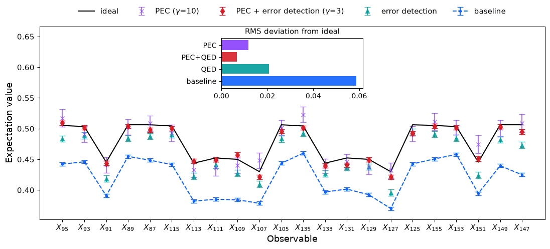
- 기댓값을 계산하고 전략을 비교합니다. QED+PEC가 실험에 영향을 미치는 노이즈를 각 방법을 단독으로 사용할 때보다 더 효과적으로 상쇄하며, PEC만 사용할 때 필요한 것보다 훨씬 적은 샷으로 수렴된 기댓값을 생성함을 확인합니다.
요구 사항
이 튜토리얼을 시작하기 전에 다음 명령을 실행하여 필요한 모든 패키지를 가져옵니다.
%pip install networkx numpy "qiskit[visualization]" "qiskit-ibm-runtime[visualization]" samplomatic qiskit-mitigation matplotlib "qiskit-noise-learning @ git+https://github.com/Qiskit/qiskit-noise-learning.git@ieee-demo-2026"
아래의 접힌 셀은 이 노트북 전체에서 사용되는 그림 헬퍼(figure helper)를 정의합니다.
그림 헬퍼를 보려면 클릭하세요
# Added by doQumentation — installs the packages this notebook needs if they are missing
import importlib.util

_needed = {"matplotlib": "matplotlib", "networkx": "networkx", "numpy": "numpy", "qiskit": "qiskit", "qiskit_ibm_runtime": "qiskit-ibm-runtime", "qiskit_mitigation": "qiskit-mitigation", "qiskit_noise_learning": "qiskit-noise-learning@git+https://github.com/Qiskit/qiskit-noise-learning.git@ieee-demo-2026", "samplomatic": "samplomatic"}
_missing = [pip for module, pip in _needed.items()
            if importlib.util.find_spec(module) is None]
# One at a time, so a package that fails to install does not block the others
for _pip in _missing:
    %pip install -q {_pip}
if not _missing:
    print("\u2713 All required packages are installed")
# Figure helpers for this notebook (collapsed): all plotting and styling lives here.
# The chip maps follow the style of Fig. 30 of arXiv:2607.25998.

from math import comb

import matplotlib.pyplot as plt
from matplotlib import cm
from matplotlib.colors import BoundaryNorm
from matplotlib.patches import Circle, Rectangle, Wedge

# one typography scheme for every figure in the notebook
plt.rcParams.update(
    {
        "font.size": 13,
        "axes.titlesize": 15,
        "axes.labelsize": 13,
        "xtick.labelsize": 11,
        "ytick.labelsize": 11,
        "legend.fontsize": 11,
    }
)

def x_labels(layout, n_data):
    """Per-observable tick labels carrying the physical qubit indices (site i = qubit i)."""
    return [f"$X_{{{layout[i]}}}$" for i in range(n_data)]

def plot_layout(backend, layout, n_data):
    """Chip cartoon of the embedding: data qubits green, check qubits orange."""
    from qiskit.visualization import plot_coupling_map

    return plot_coupling_map(
        num_qubits=backend.num_qubits,
        qubit_coordinates=None,
        coupling_map=list(backend.coupling_map.get_edges()),
        figsize=(9, 9),
        qubit_color=[
            "#4CAF50"
            if q in layout[:n_data]
            else "#FF9800"
            if q in layout[n_data:]
            else "#DDDDDD"
            for q in range(backend.num_qubits)
        ],
        qubit_size=220,
        line_width=2,
        font_size=90,
    )

def plot_exact(obs_exact, tick_labels, title):
    plt.figure(figsize=(12, 4))
    plt.plot(obs_exact, "o-")
    plt.title(title)
    plt.xticks(np.arange(len(obs_exact)), tick_labels)
    plt.xlabel("Observable")
    plt.ylabel(r"$\langle X \rangle$")
    plt.grid()

def draw_toy_circuit(
    generate_ed_ising, zz_coeff, x_coeff, include_checks=True
):
    """The boxing pipeline on a 3-plaquette-ring miniature (1 Trotter step) so the box
    structure is legible; every box carries the Twirl / InjectNoise annotations, and with
    ``include_checks`` the terminal xslow non-Markovian error check pattern is appended as in the
    production pipeline."""
    import networkx as nx
    from qiskit.circuit import ClassicalRegister
    from qiskit_mitigation.postselection import XSlowGate
    from samplomatic.transpiler import generate_boxing_pass_manager

    toy, _, _ = generate_ed_ising(nx.cycle_graph(3), 1, zz_coeff, x_coeff)
    toy.add_register(
        ClassicalRegister(3, "data"), ClassicalRegister(3, "check")
    )
    toy.barrier()
    toy.measure(range(3), range(3))
    toy.measure(range(3, 6), range(3, 6))
    toy_boxed = generate_boxing_pass_manager(
        enable_gates=True,
        enable_measures=True,
        inject_noise_targets="gates",
        inject_noise_strategy="individual_modification",
        inject_noise_site="after",
        twirling_strategy="active_circuit",
        measure_annotations="all",
    ).run(toy)
    if include_checks:
        toy_boxed.add_register(
            ClassicalRegister(3, "data_ps"), ClassicalRegister(3, "check_ps")
        )
        toy_boxed.barrier()
        for qb in range(6):
            toy_boxed.append(XSlowGate(), [qb])
        toy_boxed.measure(range(3), toy_boxed.cregs[2])
        toy_boxed.measure(range(3, 6), toy_boxed.cregs[3])
    return toy_boxed.draw("mpl", fold=-1, scale=0.6)

# --- chip-level noise maps ---------------------------------------------------------

BANDS = [1e-5, 2e-5, 3e-5, 4e-5, 6e-5, 1e-4, 2e-4, 3e-4, 4e-4, 6e-4, 1e-3]
CMAP = plt.get_cmap("YlOrBr")
NORM = BoundaryNorm(BANDS, CMAP.N, extend="both")

def _color(rate):
    return (
        "white"
        if rate < BANDS[0]
        else CMAP(NORM(min(rate, BANDS[-1] * 0.999)))
    )

def _layer_sparse(mit, weights):
    """Per-layer labelled terms from the saved run, box-local -> physical qubits."""
    phys = np.sort(mit["layout"])
    return [
        [
            (p, tuple(int(phys[q]) for q in qs if q >= 0), r)
            for p, qs, r in zip(
                mit[f"label_paulis_{i}"],
                mit[f"label_qubits_{i}"],
                w,
                strict=True,
            )
        ]
        for i, w in enumerate(weights)
    ]

def _aggregate(layers):
    """w1[qubit][P] and w2[(a,b)][PaPb]: rates summed over the 3 layers."""
    w1, w2 = {}, {}
    for terms in layers:
        for p, qs, r in terms:
            if len(qs) == 1:
                w1.setdefault(qs[0], dict.fromkeys("XYZ", 0.0))[p] += r
            else:
                (a, pa), (b, pb) = sorted(zip(qs, p, strict=True))
                w2.setdefault(
                    (a, b), {x + y: 0.0 for x in "XYZ" for y in "XYZ"}
                )[pa + pb] += r
    return w1, w2

def draw_noise_map(mit, backend, reduced=False):
    """Chip map of the learned model: X/Y/Z wheel per qubit, 3x3 two-qubit Pauli grid per
    coupler, log-banded colors, dashed outlines for unused hardware.

    With ``reduced=True``, keeps only the error terms the checks cannot see: detectability
    depends on circuit position, so each layer's 0/1 site scales are averaged over its uses.
    """
    from qiskit_ibm_runtime.visualization.embeddings import Embedding

    if reduced:
        scales = [
            mit["site_scales"][mit["site_layer"] == i].mean(axis=0)
            for i in range(3)
        ]
        weights = [mit[f"rates_{i}"] * scales[i] for i in range(3)]
        title = f"Reduced noise model ($\\gamma$ = {mit['gammas'][1]:.1f})"
    else:
        weights = [mit[f"rates_{i}"] for i in range(3)]
        title = f"Full noise model ($\\gamma$ = {mit['gammas'][0]:.0f})"
    w1, w2 = _aggregate(_layer_sparse(mit, weights))

    xy = np.array(
        [(c, -r) for r, c in Embedding.from_backend(backend).coordinates]
    )
    fig, ax = plt.subplots(figsize=(13, 7))
    for a, b in {tuple(sorted(e)) for e in backend.coupling_map.get_edges()}:
        if (
            (
                a,
                b,
            )
            in w2
        ):  # 3x3 Pauli grid laid along the bond (columns: qubit a, rows: qubit b)
            d = xy[b] - xy[a]
            u = d / np.hypot(*d)
            v = np.array([-u[1], u[0]])
            cl, cw = (np.hypot(*d) - 0.6) / 3, 0.17
            for i, Pa in enumerate("XYZ"):
                for j, Pb in enumerate("XYZ"):
                    ax.add_patch(
                        Rectangle(
                            xy[a] + u * (0.3 + i * cl) + v * ((j - 1.5) * cw),
                            cl,
                            cw,
                            angle=np.degrees(np.arctan2(u[1], u[0])),
                            facecolor=_color(w2[a, b][Pa + Pb]),
                            edgecolor="black",
                            lw=0.4,
                            zorder=2,
                        )
                    )
        else:
            ax.plot(
                *zip(xy[a], xy[b], strict=True),
                ls="--",
                lw=0.7,
                color="black",
                alpha=0.5,
                zorder=1,
            )
    for q, (xq, yq) in enumerate(xy):
        if q in w1:  # three-sector wheel: X top, Y lower left, Z lower right
            for P, t0 in (("X", 30), ("Y", 150), ("Z", 270)):
                ax.add_patch(
                    Wedge(
                        (xq, yq),
                        0.3,
                        t0,
                        t0 + 120,
                        facecolor=_color(w1[q][P]),
                        edgecolor="black",
                        lw=0.6,
                        zorder=3,
                    )
                )
            ax.annotate(
                str(q),
                (xq + 0.39, yq - 0.39),
                fontsize=9,
                color="gray",
                ha="left",
                va="top",
                zorder=4,
            )  # southeast, clear of the bond grids
        else:
            ax.add_patch(
                Circle(
                    (xq, yq),
                    0.24,
                    facecolor="none",
                    edgecolor="black",
                    ls="--",
                    lw=0.7,
                    alpha=0.5,
                    zorder=3,
                )
            )
    ux = xy[sorted(w1)]
    ax.set_xlim(ux[:, 0].min() - 2.2, ux[:, 0].max() + 2.2)
    ax.set_ylim(ux[:, 1].min() - 1.6, ux[:, 1].max() + 1.6)
    ax.set_aspect("equal")
    ax.axis("off")
    ax.set_title(title, fontsize=15)
    cb = fig.colorbar(
        cm.ScalarMappable(norm=NORM, cmap=CMAP),
        ax=ax,
        fraction=0.035,
        pad=0.02,
        extend="both",
        ticks=BANDS,
    )
    cb.set_label("coefficient (log bands; white < 1e-05)", fontsize=11)
    cb.ax.set_yticklabels(
        [f"{b:.0e}".replace("e-0", "e-") for b in BANDS], fontsize=10
    )
    _noise_map_legends(fig, ax)

def _noise_map_legends(fig, ax):
    """Weight-1 wheel and weight-2 grid keys, in a reserved band left of the lattice."""
    fig.subplots_adjust(left=0.17)
    axl = ax.inset_axes([-0.185, 0.70, 0.13, 0.24])
    for P, t0 in (("X", 30), ("Y", 150), ("Z", 270)):
        axl.add_patch(
            Wedge(
                (0.5, 0.45),
                0.38,
                t0,
                t0 + 120,
                facecolor="white",
                edgecolor="black",
                lw=0.8,
            )
        )
        axl.annotate(
            P,
            (
                0.5 + 0.2 * np.cos(np.radians(t0 + 60)),
                0.45 + 0.2 * np.sin(np.radians(t0 + 60)),
            ),
            ha="center",
            va="center",
            fontsize=9,
        )
    axl.set_title("weight-1", fontsize=10)
    axl.set_xlim(0, 1)
    axl.set_ylim(0, 1)
    axl.set_aspect("equal")
    axl.axis("off")
    axm = ax.inset_axes([-0.185, 0.32, 0.14, 0.30])
    for i, Pa in enumerate("XYZ"):
        for j, Pb in enumerate("XYZ"):
            axm.add_patch(
                Rectangle(
                    (i / 3, 1 - (j + 1) / 3),
                    1 / 3,
                    1 / 3,
                    facecolor="white",
                    edgecolor="black",
                    lw=0.6,
                )
            )
            axm.annotate(
                Pa + Pb,
                ((i + 0.5) / 3, 1 - (j + 0.5) / 3),
                ha="center",
                va="center",
                fontsize=7.5,
            )
        axm.annotate(Pa, ((i + 0.5) / 3, 1.08), ha="center", fontsize=8.5)
        axm.annotate(
            "XYZ"[i],
            (-0.13, 1 - (i + 0.5) / 3),
            ha="center",
            va="center",
            fontsize=8.5,
        )
    axm.annotate("qubit a", (0.5, 1.27), ha="center", fontsize=9)
    axm.annotate(
        "qubit b", (-0.33, 0.5), rotation=90, va="center", fontsize=9
    )
    axm.set_xlim(-0.35, 1.05)
    axm.set_ylim(-0.05, 1.35)
    axm.set_aspect("equal")
    axm.axis("off")

# --- run diagnostics ---------------------------------------------------------------

def plot_trex(trex_rescale, tick_labels):
    _fig, axt = plt.subplots(figsize=(12, 3))
    axt.stem(np.arange(len(trex_rescale)), (trex_rescale - 1) * 100)
    axt.set_xticks(np.arange(len(trex_rescale)), tick_labels)
    axt.set_xlabel("Observable")
    axt.set_ylabel("Readout correction (%)")
    axt.set_title("TREX rescale factors")
    plt.tight_layout()

def plot_postselection(mit):
    """Accepted shots per PEC randomization against a single binomial at the mean
    acceptance rate: agreement means acceptance is independent of the sampled circuit
    instance, the condition under which pooling accepted shots across randomizations
    is a consistent estimator."""
    _fig, ax = plt.subplots(figsize=(7.5, 3.8))
    counts = mit["acc_counts_post"]
    K, p = 64, counts.mean() / 64
    ks = np.arange(K + 1)
    pmf = np.array([comb(K, k) * p**k * (1 - p) ** (K - k) for k in ks])
    ax.hist(
        counts,
        bins=np.arange(-0.5, K + 1.5),
        density=True,
        alpha=0.6,
        color="#da1e28",
        label="measured",
    )
    ax.plot(ks, pmf, "k-", lw=1.5, label=f"Binomial(64, {p:.3f})")
    ax.set_xlim(-0.5, max(int(counts.max()) + 3, 20))
    ax.set_xlabel("Accepted shots per randomization")
    ax.set_ylabel("Probability")
    ax.legend()
    ax.grid(alpha=0.4)
    plt.tight_layout()

def plot_convergence(mit, obs_exact, n_data):
    """Running site-averaged estimate vs. randomizations for both PEC arms (the S5-consistent
    signed-ratio estimator, evaluated on growing prefixes of the sweep)."""

    def running(prefix):
        bits = np.squeeze(
            np.unpackbits(mit[f"data_{prefix}"], axis=-1)[..., :n_data]
            ^ mit[f"flips_{prefix}"]
        )
        mask = np.squeeze(mit[f"mask_{prefix}"])
        signs = 1 - 2 * (np.squeeze(mit[f"signs_{prefix}"]).sum(axis=-1) % 2)
        qv = (1 - 2 * bits.astype(int)) * mit["trex_rescale"]
        u = (
            (signs[:, None, None] * mask[..., None] * qv)
            .sum(axis=1)
            .mean(axis=1)
        )
        v = signs * mask.sum(axis=1)
        Rs = np.arange(500, len(u) + 1, 500)
        est, err = [], []
        for R in Rs:
            e = u[:R].sum() / v[:R].sum()
            est.append(e)
            err.append(
                np.sqrt(((u[:R] - e * v[:R]) ** 2).sum()) / abs(v[:R].sum())
            )
        return Rs, np.array(est), np.array(err)

    _fig, ax = plt.subplots(figsize=(12, 5))
    ideal_avg = float(np.mean(obs_exact))
    ax.axhline(ideal_avg, color="black", label="ideal")
    ax.fill_between(
        [-400, 24000],
        ideal_avg - 0.025,
        ideal_avg + 0.025,
        color="grey",
        alpha=0.22,
        label=r"$\pm 0.025$",
    )
    for prefix, label, color in (
        ("van", "vanilla PEC", "#8a3ffc"),
        ("post", "PEC + error detection", "#da1e28"),
    ):
        Rs, est, err = running(prefix)
        ax.errorbar(
            Rs,
            est,
            yerr=err,
            marker="o",
            linestyle="",
            markerfacecolor="none",
            color=color,
            alpha=0.85,
            capsize=3,
            label=label,
        )
    ax.set_xlim(-400, 24000)
    ax.set_ylim(ideal_avg - 0.08, ideal_avg + 0.08)
    ax.set_xlabel("# randomizations")
    ax.set_ylabel(r"Site-averaged $\langle X \rangle$")
    ax.legend(ncols=2)

def plot_final(
    obs_exact, baseline, ed, pec, post, gammas, tick_labels, title
):
    """Per-site <X> for every method, with an rms-deviation inset.
    baseline/ed/pec/post are (values, errors) pairs; gammas is (gamma, gamma_post)."""
    x = np.arange(len(obs_exact))
    _fig, ax = plt.subplots(figsize=(13, 5))
    h_ideal = ax.errorbar(
        x, obs_exact, fmt="-", capsize=4, label="ideal", color="black"
    )
    h_base = ax.errorbar(
        x,
        baseline[0],
        yerr=baseline[1],
        fmt=".--",
        capsize=4,
        label="baseline",
        color="#0f62fe",
    )
    h_ed = ax.errorbar(
        x,
        ed[0],
        yerr=ed[1],
        fmt="^",
        capsize=4,
        label="error detection",
        color="#009d9a",
        alpha=0.8,
    )
    h_pec = ax.errorbar(
        x,
        pec[0],
        yerr=pec[1],
        fmt="x",
        capsize=4,
        label=f"PEC ($\\gamma$={gammas[0]:.0f})",
        color="#8a3ffc",
        alpha=0.7,
    )
    h_post = ax.errorbar(
        x,
        post[0],
        yerr=post[1],
        fmt="d",
        capsize=4,
        label=f"PEC + error detection ($\\gamma$={gammas[1]:.0f})",
        color="#da1e28",
    )
    ax.set_xticks(x, tick_labels)
    ax.set_xlabel("Observable")
    ax.set_ylabel("Expectation value")
    # Set the y-axis range using the ideal, baseline, error detection, and PEC + error
    # detection curves, including error bars. Exclude PEC-only values when setting the
    # range so large fluctuations do not make the other curves difficult to distinguish.
    # PEC-only values may fall outside the visible range. Leave room above for the inset.
    series = [np.asarray(obs_exact)] + [
        np.asarray(v) + s * np.asarray(e)
        for v, e in (baseline, ed, post)
        for s in (-1, 1)
    ]
    lo, hi = min(a.min() for a in series), max(a.max() for a in series)
    span = max(hi - lo, 0.1)
    ax.set_ylim(lo - 0.1 * span, hi + 1.05 * span)
    # legend ordered to match the curves' vertical positions in the chart
    ax.legend(
        handles=[h_ideal, h_pec, h_post, h_ed, h_base],
        ncols=5,
        loc="lower center",
        bbox_to_anchor=(0.5, 1.02),
        frameon=False,
    )
    ax.set_title(title, pad=44)

    # inset: rows bottom-to-top so it reads top-to-bottom: PEC, PEC+ED, ED, baseline
    axi = ax.inset_axes([0.36, 0.68, 0.28, 0.26])
    methods = [
        ("baseline", baseline[0], "#0f62fe"),
        ("QED", ed[0], "#009d9a"),
        ("PEC+QED", post[0], "#da1e28"),
        ("PEC", pec[0], "#8a3ffc"),
    ]
    for k, (_nm, vals, color) in enumerate(methods):
        axi.barh(
            k,
            np.sqrt(np.mean((vals - np.array(obs_exact)) ** 2)),
            color=color,
            alpha=0.9,
        )
    axi.set_yticks(range(4), [m[0] for m in methods], fontsize=10)
    axi.set_title("RMS deviation from ideal", fontsize=11)
    axi.tick_params(labelsize=10)
    axi.patch.set_alpha(1.0)
    axi.set_zorder(5)
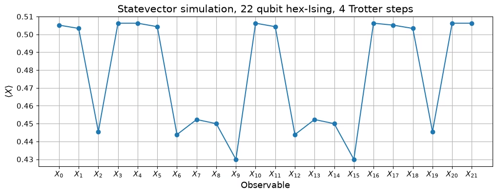
22큐비트 헥스-이징 모델의 각 사이트에 대해 를 고전적으로 시뮬레이션하기
먼저, Qiskit Statevector 클래스를 사용하여 실험의 정확한 목표 값을 시뮬레이션합니다. 우리가 풀고 있는 22큐비트 문제는 고전적으로 다룰 수 있지만, Qiskit 상태벡터 시뮬레이터는 이보다 훨씬 큰 데모로는 확장되지 않으며, 50큐비트 이상으로 확장하려면 Pauli propagation과 같은 근사 시뮬레이션 기법을 사용해야 합니다. 이 49큐비트 실험을 통해 이상적인 기댓값에 계속 접근하면서도 더 큰 규모에서 오류 검출과 오류 완화를 결합하는 것을 조사할 수 있습니다.
import warnings

import networkx as nx
import numpy as np
from qiskit.circuit import QuantumCircuit
from qiskit.quantum_info import Pauli, Statevector

# Silence two harmless upstream warnings (a Samplomatic default-change notice and a
# numpy datetime timezone notice from the noise-learning circuit generator)
warnings.filterwarnings(
    "ignore", message="The default of the 'inject_noise_site'"
)
warnings.filterwarnings(
    "ignore", message="no explicit representation of timezones"
)

# Hexagonal lattice
data_graph = nx.convert_node_labels_to_integers(
    nx.hexagonal_lattice_graph(2, 3)
)

# Number of Trotter steps and rotation angles
depth = 4
zz_coeff = -np.pi / 4
x_coeff = 3 * np.pi / 8
n_data = data_graph.order()
n_checks = data_graph.size()
n_qubits = n_data + n_checks

qc_data = QuantumCircuit(n_data)
qc_data.h(range(n_data))
for _ in range(depth):
    for edge in data_graph.edges:
        qc_data.rzz(zz_coeff, *edge)
    qc_data.rx(x_coeff, range(n_data))
psi_exact = Statevector(qc_data)

# X on site i = qubit i
observables = ["I" * (n_data - 1 - i) + "X" + "I" * i for i in range(n_data)]
obs_exact = [psi_exact.expectation_value(Pauli(o)).real for o in observables]

plot_exact(
    obs_exact,
    x_labels(range(n_data), n_data),
    f"Statevector simulation, {n_data} qubit hex-Ising, {depth} Trotter steps",
)
49큐비트 오류 검출 헥스-이징 모델을 양자 회로로 구현하고 QPU 백엔드로 트랜스파일하기
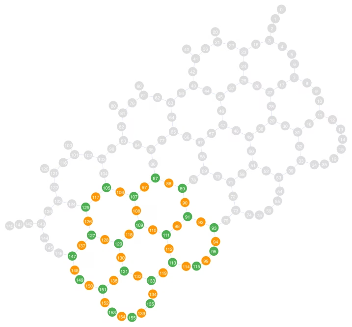
이 회로는 육각 격자(hexagonal lattice)에서 22큐비트 횡자기장 이징 해밀토니안(transverse-field Ising Hamiltonian)의 4개 트로터 단계를 시뮬레이션합니다. 22개의 데이터 큐비트는 Heron r3 QPU인 ibm_boston의 49큐비트 헤비-헥스(heavy-hex) 서브그래프에 임베딩됩니다. 27개의 보조(ancilla) 큐비트는 두 가지 목적으로 사용됩니다. 이징 큐비트 간의 얽힘을 매개하는 것과 회로 실행 중 논리 오류를 검출하는 것입니다. 회로의 얽힘 레이어는 매개 큐비트가 최종 측정 전에 바닥 상태 로 돌아가도록 구현되어 있습니다. 하나 이상의 매개 큐비트가 로 측정되면 해당 샘플이 논리 오류로 손상되었음을 나타냅니다. 이러한 샘플을 버리면 샘플링된 분포의 충실도를 향상시킬 수 있습니다.
아래 그래프에서 녹색 큐비트는 22개의 이징 큐비트를 나타내고, 주황색 큐비트는 27개의 매개 큐비트를 나타냅니다.
from qiskit.circuit import ClassicalRegister
from qiskit.transpiler import generate_preset_pass_manager
from qiskit_ibm_runtime import QiskitRuntimeService

backend_name = "ibm_boston"

def generate_ed_ising(graph, depth, zz_coeff, x_coeff):
    """Build the mediated error-detecting Ising circuit for data-qubit `graph`; returns (circuit, CZ layers, hardware graph)."""
    hw_graph = nx.Graph()
    for i, (a, b) in enumerate(graph.edges()):
        hw_graph.add_edges_from(
            [(a, i + graph.order()), (b, i + graph.order())]
        )
    coloring = nx.coloring.greedy_color(
        nx.line_graph(hw_graph), strategy="DSATUR"
    )
    layers_coupling = [
        [e for e, c in coloring.items() if c == i]
        for i in set(coloring.values())
    ]
    circuit = QuantumCircuit(hw_graph.order())
    circuit.h(range(hw_graph.order()))
    for _ in range(depth):
        for angle, qubits in (
            (zz_coeff, range(graph.order(), hw_graph.order())),
            (x_coeff, range(graph.order())),
        ):
            circuit.barrier()
            for layer in layers_coupling:
                for edge in layer:
                    circuit.cz(*edge)
            circuit.barrier()
            circuit.rx(angle, qubits)
    circuit.barrier()
    circuit.h(range(graph.order(), hw_graph.order()))
    return circuit, layers_coupling, hw_graph

service = QiskitRuntimeService()
backend = service.backend(backend_name)

circuit, layers_coupling, hw_graph = generate_ed_ising(
    data_graph, depth, zz_coeff, x_coeff
)

circ_meas = circuit.copy()
data_reg, check_reg = (
    ClassicalRegister(n_data, "data"),
    ClassicalRegister(n_checks, "check"),
)
circ_meas.add_register(data_reg, check_reg)
circ_meas.barrier()
circ_meas.measure(range(n_data), data_reg)
circ_meas.measure(range(n_data, n_qubits), check_reg)

# Physical qubits hosting the 22 Ising sites on ibm_boston, one heavy-hex row per lattice chain;
# the mediator for each edge is the physical qubit sitting between its two data qubits
data_layout = [
    *[95, 93, 91, 89, 87],
    *[115, 113, 111, 109, 107, 105],
    *[135, 133, 131, 129, 127, 125],
    *[155, 153, 151, 149, 147],
]
coupling_graph = nx.Graph(list(backend.coupling_map.get_edges()))
layout = data_layout + [
    next(
        iter(
            nx.common_neighbors(
                coupling_graph, data_layout[a], data_layout[b]
            )
        )
    )
    for a, b in data_graph.edges()
]

circ_trans = generate_preset_pass_manager(
    backend=backend, optimization_level=1, initial_layout=layout
).run(circ_meas)

plot_layout(backend, layout, n_data)
samplomatic으로 회로의 얽힘 레이어 지정하기.
Samplomatic의 generate_boxing_pass_manager 패스는 회로의 얽힘 레이어를 Pauli 트위링과 PEC 노이즈 주입을 위한 주석이 달린 박스로 그룹화합니다. 그 결과로 생성된 템플릿 회로와 샘플렉스(samplex, 템플릿 회로의 트위링과 노이즈 주입을 지정하는 매개변수 분포)는 모든 노이즈 학습 및 샘플링 QPU 실험을 정의하고 실행하는 데 사용됩니다. 측정 박스에는 ChangeBasis 주석도 있어서, 데이터 큐비트를 X 기저에서 측정하는 회전이 회로에 고정되어 있지 않고 샘플링 시점에 입력으로 샘플렉스에 제공됩니다.
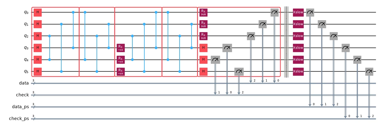
아래에서는 박스화된 회로의 구조를 시각화할 수 있도록 동일한 박스화 패스를 오류 검출 이징 회로의 작은 버전에 적용합니다.
from samplomatic.builders import build
from samplomatic.transpiler import generate_boxing_pass_manager
from samplomatic.utils import find_unique_box_instructions

boxed = generate_boxing_pass_manager(
    enable_gates=True,
    enable_measures=True,
    inject_noise_targets="gates",
    inject_noise_strategy="individual_modification",
    inject_noise_site="after",
    twirling_strategy="active_circuit",
    measure_annotations="all",
).run(circ_trans)
template, samplex = build(boxed)
unique_instructions = find_unique_box_instructions(
    boxed, normalize_annotations=None, undress_boxes=True
)

# Measure X on the data qubits and Z on the mediators
basis_key = next(
    s.name
    for s in samplex.inputs().get_specs()
    if s.name.startswith("basis_changes.")
)
meas_basis = np.array(
    [2 if q in set(layout[:n_data]) else 1 for q in sorted(layout)],
    dtype=np.uint8,
)

draw_toy_circuit(generate_ed_ising, zz_coeff, x_coeff, include_checks=False)

회로에 비마르코프 오류 검사 추가하기
다음으로, 학습 프로토콜에서 모델링되지 않은 노이즈로부터 보호하기 위해 회로에 비마르코프 오류 검사를 추가합니다. 이 검사는 긴 펄스의 비트 플립을 구현하고 큐비트가 한 고전 상태에서 다른 상태로 올바르게 이동했는지 확인하는 방식으로 작동합니다. 한 에지의 두 큐비트가 모두 검사에 실패하면 해당 샘플은 버려집니다. 비마르코프 오류 검사는 회로의 시작이나 끝(또는 둘 다)에서 사용할 수 있습니다. 여기서는 끝에서만 사용합니다. 또한 회로에 인접한 사용되지 않는 "스펙테이터(spectator)" 큐비트에도 검사를 배치하여, 이 검사가 검출하도록 설계된 노이즈에 대한 커버리지를 넓힙니다.
대칭 검사와 마찬가지로 이것 역시 사후 선택(postselection)의 한 형태이므로, 이러한 기법들을 결합할 때 사후 선택 비율의 감소를 고려해야 함을 기억하세요. 구체적으로, 이고 라면, 하나의 논리 샘플을 복구하는 데 약 개의 노이즈 샘플이 필요합니다.
from qiskit.transpiler import PassManager
from qiskit_mitigation.postselection import PostSelector
from qiskit_mitigation.postselection.passes import (
    AddPostCircuitNonMarkovianErrorChecks,
    AddSpectatorPostCircuitNonMarkovianErrorChecks,
)

add_checks = PassManager(
    [
        AddPostCircuitNonMarkovianErrorChecks(x_pulse_type="xslow"),
        AddSpectatorPostCircuitNonMarkovianErrorChecks(
            backend.coupling_map, x_pulse_type="xslow"
        ),
    ]
)
template_checked = add_checks.run(template)
selector = PostSelector.from_circuit(template_checked, backend.coupling_map)

draw_toy_circuit(generate_ed_ising, zz_coeff, x_coeff, include_checks=True)
49큐비트 검사된 이징 회로의 게이트 및 판독 노이즈 학습하기
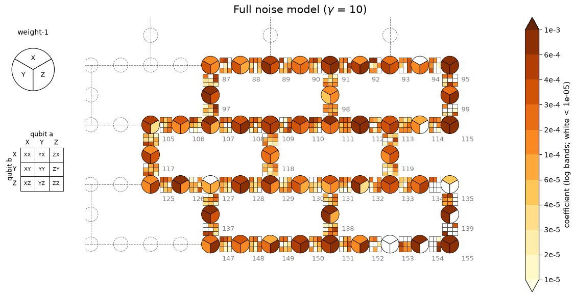
노이즈를 완화하려면 노이즈가 얽힘 게이트에 어떻게 영향을 미치는지 모델링해야 합니다. 여기서는 qiskit-noise-learning을 사용하여 회로의 세 가지 고유한 얽힘 레이어 각각에 대한 Pauli-Lindblad 노이즈 모델을 학습합니다. 이후 이 노이즈 모델에서 대칭 검사로 검출 가능한 오류 생성자(error generator)를 제거하고, 남은 노이즈 채널만 PEC로 완화합니다. 아래 지도는 QPU에서 학습된 세 개의 레이어를 보여줍니다. 각 큐비트는 가중치-1 X/Y/Z 비율의 원형(wheel)으로, 각 커플러는 해당 쌍의 가중치-2 Pauli 비율의 3×3 격자로 표시됩니다. 값이 이라는 것은 의 샘플링 오버헤드를 의미합니다.
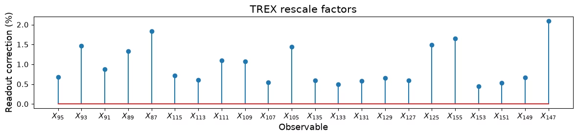
판독(TREX) 보정은 노이즈 학습 피팅의 SPAM 경로에서 직접 얻어집니다. QPU 노이즈 지도 아래의 스템 플롯은 관측 가능량별 TREX 재조정 계수를 보여줍니다.
from qiskit.quantum_info import PauliLindbladMap, QubitSparsePauli
from qiskit_ibm_runtime import Executor, Session
from qiskit_ibm_runtime.quantum_program import QuantumProgram
from qiskit_mitigation.trex import TREX
from qiskit_noise_learning.analysis import (
    ComputeObservables,
    CurveFitObservables,
    FlipPostSelect,
    LeastSquaresSolve,
)
from qiskit_noise_learning.circuit_generator import ExecutorCircuitGenerator
from qiskit_noise_learning.experiment_builder import (
    BindFragmentDepths,
    CompleteSequences,
    EvenDepthVanillaPaths,
    Experiment,
    GenerateInstructionSequences,
    IdentifyRelations,
    MergeInstructionSequences,
    SPAMPaths,
    VanillaInstructionSequences,
)
from qiskit_noise_learning.gate_sets import QiskitGateSet
from qiskit_noise_learning.models import PauliLindbladModel
from qiskit_noise_learning.models.utils import split_pauli_lindblad_model
from samplomatic.annotations import InjectNoise
from samplomatic.utils import get_annotation

gate_set = QiskitGateSet(
    target=backend.target,
    qubit_subset=sorted(
        {
            boxed.find_bit(q).index
            for i in unique_instructions
            for q in i.qubits
        }
    ),
)
ref_to_qubits = {}
for inst in unique_instructions:
    if ann := get_annotation(inst.operation, InjectNoise):
        gate_set.add_box_as_gate(inst, name=ann.ref)
        ref_to_qubits[ann.ref] = sorted(
            boxed.find_bit(q).index for q in inst.qubits
        )

fidelity_model = PauliLindbladModel.k_local(
    gate_set, gate_k={**{r: 2 for r in ref_to_qubits}, "M": 1, "P": 1}
)
experiment = (
    EvenDepthVanillaPaths()
    + VanillaInstructionSequences()
    + IdentifyRelations()
    + SPAMPaths()
    + GenerateInstructionSequences()
    + MergeInstructionSequences()
    + CompleteSequences()
    + BindFragmentDepths([2, 4, 8, 12])
).run(Experiment(fidelity_model=fidelity_model, shots=384, randomizations=64))

circuit_generator = ExecutorCircuitGenerator(
    gate_set, pass_manager=add_checks
)
program_learn, data_mapper = circuit_generator.generate(experiment)

session = Session(backend)
executor_options = {"environment": {"job_tags": ["TUT_PECLNM"]}}
fit = circuit_generator.collect(
    Executor(session, options=executor_options).run(program_learn).result(),
    data_mapper,
)
fit = (
    FlipPostSelect()
    + ComputeObservables()
    + CurveFitObservables()
    + LeastSquaresSolve()
).run(fit)
print(
    "learning shots removed by checks:",
    f"{float(fit.raw_data.datatree['0']['data_mask'].mean()):.4f}",
)

# TREX factors from the fit's SPAM paths: the fit only identifies the product of
# state-prep and measurement error, so hand TREX the composition of the two maps
spam = fidelity_model.to_pauli_lindblad_maps(
    fit.model_data, include_spam=True
)
spam_map = spam["P"].compose(spam["M"])
z_terms = [
    QubitSparsePauli(("Z", [layout[i]]), num_qubits=backend.num_qubits)
    for i in range(n_data)
]
trex_rescale = np.array(
    [TREX.calculate_trex_factor(spam_map, z) for z in z_terms]
)

# learned maps come back in backend qubit indexing; samplex wants box-local order
plm = split_pauli_lindblad_model(fit.model).model
noise_maps = {}
for ref, m in plm.to_pauli_lindblad_maps(fit.model_data).items():
    box = ref_to_qubits[ref]
    noise_maps[ref] = PauliLindbladMap.from_sparse_list(
        [
            (p, tuple(box.index(q) for q in qs), r)
            for p, qs, r in m.to_sparse_list()
        ],
        num_qubits=len(box),
    )
# Full-PEC cost: each learned layer acts twice per Trotter step (compute + uncompute)
gamma = float(
    np.exp(2 * depth * sum(2 * sum(m.rates) for m in noise_maps.values()))
)

# Collect the learned model in the form the figure helpers expect
mit = dict(
    **{
        f"rates_{i}": np.asarray(m.rates)
        for i, m in enumerate(noise_maps.values())
    },
    **{
        f"label_paulis_{i}": np.array([p for p, _, _ in m.to_sparse_list()])
        for i, m in enumerate(noise_maps.values())
    },
    **{
        f"label_qubits_{i}": np.array(
            [
                list(qs) + [-1] * (2 - len(qs))
                for _, qs, _ in m.to_sparse_list()
            ]
        )
        for i, m in enumerate(noise_maps.values())
    },
    layout=np.array(layout),
    trex_rescale=trex_rescale,
    gammas=np.array([gamma, np.nan]),
)
draw_noise_map(mit, backend)
plot_trex(mit["trex_rescale"], x_labels(layout, n_data))
learning shots removed by checks: 0.2393
대칭 검사로 검출 가능한 항을 노이즈 모델에서 제거하기
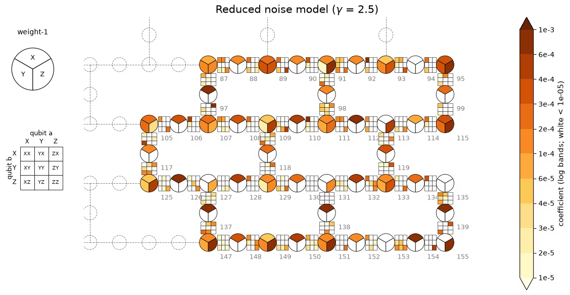
각 대칭 검사는 노이즈 모델의 오류 생성자 중 일부 부분집합을 검출할 수 있으며, 이는 해당 오류를 완화할 필요가 없음을 의미합니다. 여기서는 qiskit_mitigation의 create_postselected_noise_mask 함수를 사용하여 검출 가능한 노이즈 생성자에 대한 마스크를 생성합니다. 이 마스크는 PEC를 수행하기 전에 검출 가능한 항을 노이즈 모델에서 제거하는 데 사용됩니다. 위의 노이즈 모델 지도에서 보여지듯이, 제거된 노이즈 모델에 대해 PEC를 수행하면 전체 노이즈 모델에 PEC를 수행하는 데 필요한 샘플링 비용의 일부만으로 수렴된 기댓값을 얻을 수 있습니다.
아래 지도는 위의 학습된 모델과 동일한 색상 스케일로 그려졌으며, 검사가 검출할 수 없는 오류 생성자만 남긴 것입니다. 많은 수의 오류 생성자가 모델에서 제거되었고, 샘플링 오버헤드가 크게 줄어든 것을 볼 수 있습니다. 제거된 노이즈 모델에서 PEC를 실행하는 데 필요한 샘플링 오버헤드는 이며, 이는 전체 노이즈 채널을 완화하는 데 필요한 오버헤드보다 약 16배 감소한 것입니다.
from qiskit.quantum_info import Pauli
from qiskit_mitigation.noise import create_postselected_noise_mask

SHOTS_PER_RAND = 64  # shots per PEC randomization
N_RAND = 23_054  # PEC randomizations per experiment
MAX_PAIR_RATE = 0.02  # Max value of any coupler's summed two-qubit error rate

# The detectors are virtual Pauli-Z's representing the measurements on the mediator qubits
# We can find the set of detectable noise generators in the model for each detector by conjugating
# it backward through the circuit and calculating what generators it anti-commutes with.
detectors = [
    Pauli("I" * (boxed.num_qubits - 1 - q) + "Z" + "I" * q)
    for q in layout[n_data:]
]
# Detectable generators are handled by postselection; prune them from the model for PEC
local_scales, gamma2_post = create_postselected_noise_mask(
    boxed, noise_maps, detectors
)
gamma_post = gamma2_post**0.5
print(f"gamma PEC {gamma:.2f} | gamma QED+PEC {gamma_post:.2f}")

# Kill the job if any coupler's summed rate exceeds MAX_PAIR_RATE
pair_lam = {}
for m in noise_maps.values():
    for _, qs, r in m.to_sparse_list():
        if len(qs) == 2:
            pair_lam[tuple(sorted(qs))] = (
                pair_lam.get(tuple(sorted(qs)), 0.0) + r
            )
assert (
    max(pair_lam.values()) < MAX_PAIR_RATE
), f"kill: degraded coupler {max(pair_lam, key=pair_lam.get)}"

# Detectability depends on circuit position, so record each site's 0/1 scales by layer
site_ref = {
    a.modifier_ref: a.ref
    for inst in boxed.data
    if inst.operation.name == "box"
    and (a := get_annotation(inst.operation, InjectNoise))
    and a.ref
}
sites = sorted(local_scales, key=lambda s: int(s[1:]))
mit["site_scales"] = np.stack([local_scales[s] for s in sites])
mit["site_layer"] = np.array(
    [list(noise_maps).index(site_ref[s]) for s in sites]
)
mit["gammas"] = np.array([gamma, gamma_post])
draw_noise_map(mit, backend, reduced=True)
gamma PEC 10.08 | gamma QED+PEC 2.52
오류 검출 회로 샘플링하기
여기서는 49큐비트 오류 검출 이징 회로를 샘플링합니다. Pauli 트위링과 비마르코프 오류 검사를 활성화하지만 PEC 샘플링은 수행하지 않습니다. 이 샘플들을 사용하여 기준 기댓값과 오류 검출만 적용한 기댓값을 모두 계산합니다.
# Baseline = the ED+PEC template itself at noise scale 0, i.e. twirling only
program_tw = QuantumProgram(shots=100)
program_tw.append_samplex_item(
    template_checked,
    samplex=samplex,
    shape=(1000, 1),
    samplex_arguments={
        "pauli_lindblad_maps": dict(noise_maps),
        basis_key: meas_basis,
        **{f"noise_scales.{k}": 0.0 for k in local_scales},
    },
)
job_tw = Executor(session, options=executor_options).run(program_tw)
PEC를 사용해 오류 검출 회로 샘플링하기
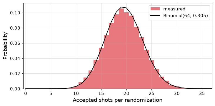
이제 다시 샘플링하며, 대칭 검사가 검출할 수 없는 노이즈를 완화하기 위해 PEC 무작위화(randomization)를 포함합니다. 이 샘플들은 오류 검출과 PEC를 결합하여 기댓값을 계산하는 데 사용됩니다. 아래에서는 PEC 무작위화당 사후 선택을 통과한 샷을 평균 통과율의 이항 분포와 비교하여 플롯합니다. QED+PEC는 모든 매개 큐비트의 측정과 교환(commute)하는 검출 불가능한 Pauli만 주입하기 때문에, 통과 여부는 샘플링된 회로 인스턴스와 상관관계가 없음을 알 수 있습니다.
def launch(session, template, samplex, samplex_args, n_rand, shots_per_rand):
    """Sample `n_rand` randomizations of `template` on `session` in <=100k-randomization jobs; returns the jobs."""
    jobs = []
    for start in range(0, n_rand, 100_000):
        program = QuantumProgram(shots=shots_per_rand)
        program.append_samplex_item(
            template,
            samplex=samplex,
            samplex_arguments=samplex_args,
            shape=(min(100_000, n_rand - start), 1),
        )
        jobs.append(Executor(session, options=executor_options).run(program))
    return jobs

# Reduced PEC
args_post = {
    "pauli_lindblad_maps": dict(noise_maps),
    basis_key: meas_basis,
    **{f"noise_scales.{k}": -1.0 for k in local_scales},
    **{f"local_scales.{k}": v for k, v in local_scales.items()},
}
# PEC on the full noise model
args_van = {
    "pauli_lindblad_maps": dict(noise_maps),
    basis_key: meas_basis,
    **{f"noise_scales.{k}": -1.0 for k in local_scales},
}

# Run sampling jobs
jobs = launch(
    session, template_checked, samplex, args_post, N_RAND, SHOTS_PER_RAND
)
jobs_van = launch(
    session, template_checked, samplex, args_van, N_RAND, SHOTS_PER_RAND
)
outs = [j.result()[0] for j in jobs]
outs_van = [j.result()[0] for j in jobs_van]
(out_tw,) = job_tw.result()
session.close()
샘플을 수집하고, PEC 무작위화가 매개 큐비트의 측정과 교환하며 사후 선택 통계에 영향을 미치지 않음을 확인합니다.
def bitflip_mask(out, selector):
    """Per-shot True/False for job result `out`: shot passes `selector`'s non-Markovian error checks."""
    regs = {
        k: np.asarray(out[k])
        for k in out
        if not k.startswith(("measurement_flips", "pauli_signs"))
    }
    return selector.compute_mask(regs, "edge", mode="post")

def symmetry_mask(out):
    """Per-shot True/False for job result `out`: every twirl-corrected symmetry check reads 0."""
    return ~(
        np.asarray(out["check"]) ^ np.asarray(out["measurement_flips.check"])
    ).any(axis=-1)

def keep_mask(out, selector):
    """Per-shot True/False for job result `out`: shot passes both check types."""
    return symmetry_mask(out) & bitflip_mask(out, selector)

def fracs(out_list, selector):
    """Fractions of shots across the job results in `out_list` passing [no, non-Markovian error, symmetry, both] checks."""
    bf = np.concatenate([bitflip_mask(o, selector) for o in out_list])
    sy = np.concatenate([symmetry_mask(o) for o in out_list])
    return [1.0, bf.mean(), sy.mean(), (bf & sy).mean()]

mask_post = np.concatenate([keep_mask(o, selector) for o in outs])

# Collect the sampled data alongside the learned model, in the form the figure helpers expect
mit.update(
    ps_fracs=np.array(
        [
            fracs([out_tw], selector),
            fracs(outs_van, selector),
            fracs(outs, selector),
        ]
    ),
    acc_counts_post=np.squeeze(mask_post).sum(axis=-1),
    data_tw=np.asarray(out_tw["data"]),
    flips_tw=np.asarray(out_tw["measurement_flips.data"]),
    mask_tw=keep_mask(out_tw, selector),
    data_post=np.packbits(
        np.concatenate([np.asarray(o["data"]) for o in outs]), axis=-1
    ),
    flips_post=np.concatenate(
        [np.asarray(o["measurement_flips.data"]) for o in outs]
    ),
    signs_post=np.concatenate([np.asarray(o["pauli_signs"]) for o in outs]),
    mask_post=mask_post,
    data_van=np.packbits(
        np.concatenate([np.asarray(o["data"]) for o in outs_van]), axis=-1
    ),
    flips_van=np.concatenate(
        [np.asarray(o["measurement_flips.data"]) for o in outs_van]
    ),
    signs_van=np.concatenate(
        [np.asarray(o["pauli_signs"]) for o in outs_van]
    ),
    mask_van=np.concatenate([bitflip_mask(o, selector) for o in outs_van]),
)

# Plot the PEC bias check
plot_postselection(mit)
기댓값 계산 및 전략 비교하기
마지막으로, 측정 플립, 사후 선택 마스크, TREX 재조정 계수, 유사 확률(quasi-probability) 부호를 적용해주는 qiskit-mitigation의 executor_expectation_values 헬퍼 함수를 사용하여 모든 기댓값을 계산합니다.
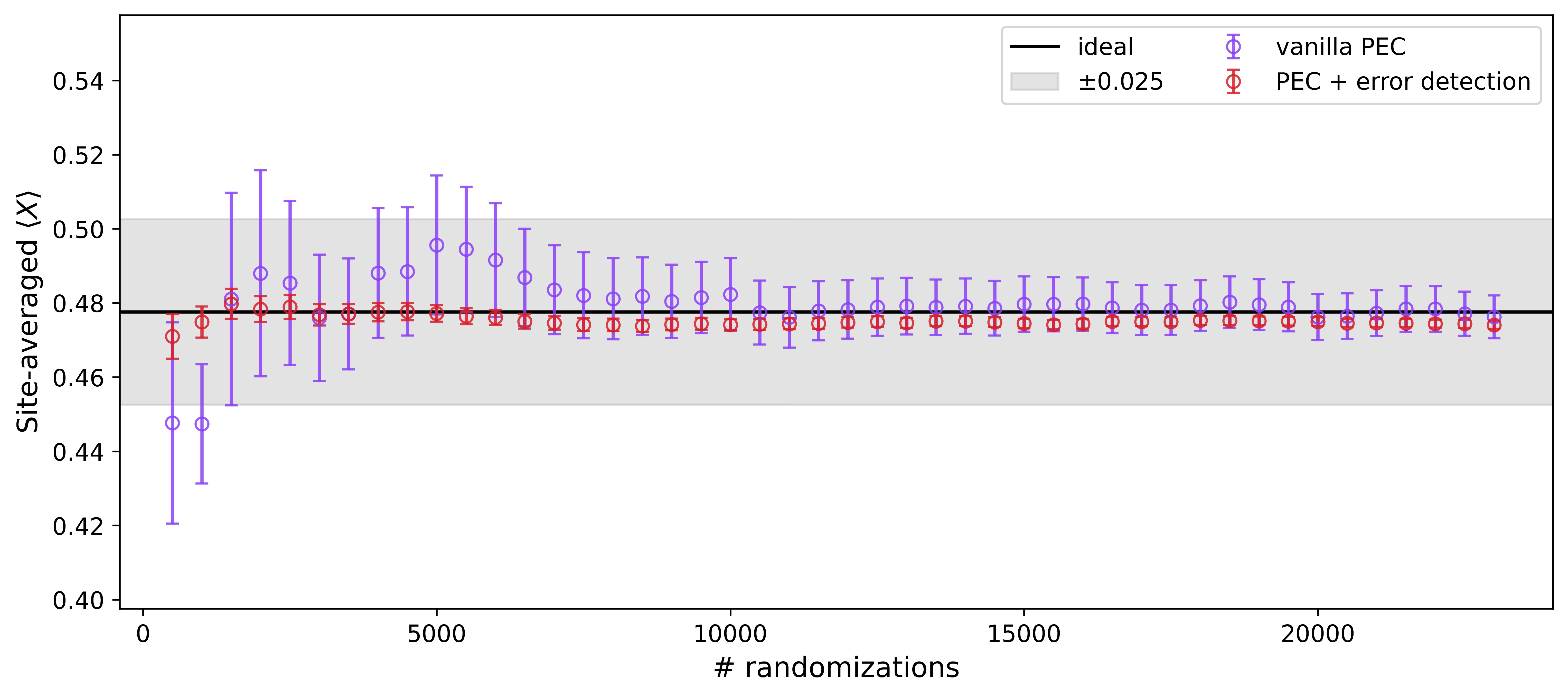
상단 차트: 두 PEC 변형 모두 수렴하지만, QED+PEC는 더 적은 무작위화로 더 좁은 오차 막대와 함께 대역에 도달합니다. QED+PEC 계산의 잔여 편향(residual bias)은 0.01 미만이며, 이는 노이즈 모델 불일치, 시간에 따른 큐비트 드리프트, 모델링되지 않은 노이즈원의 영향이 복합적으로 작용한 것으로 볼 수 있습니다.
하단 차트: 두 PEC 변형 모두 무작위화당 동일한 샷 수를 사용하여 무작위화가 누적됨에 따른 사이트 평균 의 누적 추정치입니다. PEC + 오류 검출은 수천 번의 무작위화 내에 대역 안으로 안정화되지만, 전체 샘플링 오버헤드를 감수하는 PEC 단독 방식은 수렴하는 데 훨씬 더 많은 무작위화가 필요합니다.
from qiskit.quantum_info import SparsePauliOp
from qiskit_mitigation.utils import executor_expectation_values

gamma, gamma_post = mit["gammas"]
basis_map = {Pauli("X" * n_data): [SparsePauliOp(o) for o in observables]}
rescale = dict(zip(observables, mit["trex_rescale"], strict=True))

def evs(bits, basis_map, **kwargs):
    """Per-site (means, standard errors) from boolean shot data `bits` of shape (rands, 1, shots, n_data)."""
    out = executor_expectation_values(
        bits, basis_map, None, avg_axis=(0, 1), **kwargs
    )
    return np.array([m for m, _ in out]).ravel(), np.sqrt(
        [v for _, v in out]
    ).ravel()

def unpack(mit, prefix, n_data):
    """Restore `mit[f"data_\{prefix\}"]` from packed bytes to booleans of shape (rands, 1, shots, n_data)."""
    return np.unpackbits(mit[f"data_{prefix}"], axis=-1)[..., :n_data].astype(
        bool
    )

unmit_tw, unmit_tw_err = evs(
    mit["data_tw"], basis_map, measurement_flips=mit["flips_tw"]
)
ed_tw, ed_tw_err = evs(
    mit["data_tw"],
    basis_map,
    measurement_flips=mit["flips_tw"],
    postselect_mask=mit["mask_tw"],
    rescale_factors=rescale,
)
post, post_err = evs(
    unpack(mit, "post", n_data),
    basis_map,
    measurement_flips=mit["flips_post"],
    pauli_signs=mit["signs_post"],
    postselect_mask=mit["mask_post"],
    rescale_factors=rescale,
)
pec, pec_err = evs(
    unpack(mit, "van", n_data),
    basis_map,
    measurement_flips=mit["flips_van"],
    pauli_signs=mit["signs_van"],
    postselect_mask=mit["mask_van"],
    rescale_factors=rescale,
)

# effective ED+PEC overhead measured from the data: accepted shots per signed accepted shot
signs_post = 1 - 2 * (np.squeeze(mit["signs_post"]).sum(axis=-1) % 2)
gamma_eff = (
    mit["mask_post"].sum()
    / (signs_post * np.squeeze(mit["mask_post"]).sum(axis=-1)).sum()
)

print(
    f"gamma PEC {gamma:.2f} | gamma QED+PEC {gamma_post:.2f} (model) / {gamma_eff:.2f} (data) | "
    f"QED survival {mit['mask_tw'].mean():.3f} | QED+PEC survival {mit['mask_post'].mean():.3f} | "
    f"mean QED+PEC err {post_err.mean():.4f}"
)
plot_final(
    obs_exact,
    (unmit_tw, unmit_tw_err),
    (ed_tw, ed_tw_err),
    (pec, pec_err),
    (post, post_err),
    (gamma, gamma_post),
    x_labels(layout, n_data),
    "",
)
gamma PEC 10.08 | gamma QED+PEC 2.52 (model) / 2.51 (data) | QED survival 0.304 | QED+PEC survival 0.305 | mean QED+PEC err 0.0037
plot_convergence(mit, obs_exact, n_data)