전파된 노이즈 흡수(PNA)로 기댓값 개선하기

사용 예상 시간: Heron 프로세서에서 10분 (참고: 이는 예상치일 뿐이며 실제 실행 시간은 다를 수 있습니다.)

학습 목표

• 전파된 노이즈 흡수(PNA)가 무엇인지, 그리고 학습된 역노이즈 채널을 측정 관측량에 흡수시켜 2-Qubit 게이트 노이즈를 어떻게 완화하는지

• samplomatic을 사용하여 트월링, 기저 변경, 노이즈 주입을 위해 회로 레이어를 박싱하고 주석을 다는 방법

• [NoiseLearnerV3](/guides/directed-execution-model#noiselearnerv3)로 레이어 노이즈를 학습하고 이를 qiskit-addon-pna를 이용해 노이즈 완화 관측량으로 전파하는 방법

• qiskit-ibm-runtime의 QuantumProgram 및 Executor 클래스를 이용하여 무작위화된 회로를 샘플링하고 PNA를 TREX 및 후선택과 결합하는 방법

사전 준비 사항

• Qiskit 패턴 워크플로우

• 관측량의 기댓값을 계산하기 위해 Estimator 프리미티브를 사용하는 방법

• Estimator 프리미티브와 오류 완화 옵션 결합하기에서 다룬 Pauli 트월링 및 TREX와 같은 오류 완화 기법

배경

이 튜토리얼에서는 노이즈가 있는 양자 실험에서 기댓값 추정을 개선하기 위해 Qiskit의 고급 오류 완화 도구를 활용하는 방법을 보여줍니다.

전파된 노이즈 흡수(PNA)란 무엇인가요?

전파된 노이즈 흡수는 2-Qubit 게이트에 영향을 미치는 역노이즈 채널을 통해 관측량을 전파함으로써 게이트 오류를 완화하는 기법으로, 노이즈 완화 관측량을 생성합니다.

완전한 결함 허용을 요구하지 않고도 노이즈가 있는 양자 하드웨어에서 유용한 기댓값을 추출하기 위해 양자 오류 완화를 사용할 수 있습니다. PNA는 특히 회로 연산을 수정하는 대신 관측량 자체에 노이즈 효과를 흡수시키는 데 중점을 둡니다.

양자 회로의 각 노이즈가 있는 게이트는 이상적인 게이트 다음에 노이즈 채널이 뒤따르는 것으로 모델링할 수 있습니다. PNA는 이러한 노이즈 채널을 학습하거나 특성화하고 그 역을 정의합니다. 역 연산을 하드웨어 실행에 삽입하는 대신(일반적으로 이는 실현 불가능함), PNA는 역노이즈 채널을 회로를 통해 순방향으로 전파하여 관측량에 적용합니다. 이 과정은 관측량 $O$를 새로운 연산자 $\tilde{O}$로 변환하여, 노이즈가 있는 회로에서 $\tilde{O}$를 측정하면 이상적인 노이즈 없는 회로에서 $O$를 측정한 것과 동일한 기댓값을 얻을 수 있게 합니다.

이는 다음과 같이 요약할 수 있습니다:

1. 각 노이즈가 있는 게이트 $u_i$를 이상적인 연산 다음에 노이즈 채널 $\Lambda_i$가 뒤따르는 것으로 모델링합니다.
2. 노이즈 특성화 도구를 사용하여 각 $\Lambda_i$를 학습하거나 추정합니다.
3. Pauli 전달 기법을 사용하여 역노이즈 맵 $\Lambda_i^{-1}$을 정의하고 회로를 통해 순방향으로 전파합니다.
4. 이러한 역을 관측량에 흡수시켜, 노이즈가 완화된 연산자 $\tilde{O}$를 얻습니다.

노이즈가 파울리 채널(또는 더 일반적으로 희소 파울리-린드블라드 채널)로 기술될 경우, 이 전파는 파울리 전파를 사용하여 효율적으로 수행할 수 있습니다. 파울리 전파는 계산 복잡도를 제어하면서, 역노이즈 채널이 클리퍼드 및 비클리퍼드 연산의 레이어를 통과할 때 어떻게 변환되는지를 근사하는 프레임워크를 제공합니다.

완화 작업을 관측량으로 옮김으로써, PNA는 회로에 물리적 보정 연산을 삽입할 때 발생하는 큰 샘플링 오버헤드를 피할 수 있습니다. 대신, 원래의 노이즈가 있는 회로가 실행되며, 관측량은 그 기댓값이 노이즈의 효과를 상쇄하는 새로운 연산자 $\tilde{O}$로 변환됩니다.

PNA 워크플로우

이 과정은 다음과 같은 개념적 단계를 통해 이해할 수 있습니다. 첫 번째 개략도는 표준적인 노이즈가 있는 실험을 보여줍니다.

노이즈 모델을 학습하면 그 역을 적용하여 노이즈를 상쇄할 수 있습니다.

확률적 오류 상쇄(PEC)에서처럼 QPU에서 샘플링하여 역노이즈 채널을 구현하는 대신, Pauli 전파를 사용하여 측정된 관측량에 이를 고전적으로 적용합니다. 그 결과 얻어진 관측량은 측정 시 학습된 게이트 노이즈를 효과적으로 완화합니다.

Samplomatic과 Executor를 이용한 모듈식 오류 완화

PNA 접근 방식은 Qiskit의 모듈식 오류 완화 아키텍처를 기반으로 합니다. 이 아키텍처는 samplomatic 라이브러리를 QuantumProgram 및 Executor 클래스(qiskit-ibm-runtime v0.47.0에서 Qiskit Runtime에 추가됨)와 함께 사용하여, 전파된 노이즈 흡수와 Pauli 트월링 같은 기법을 서로 다른 실험 간에 조합 가능하고 재사용 가능하게 만듭니다.

완화 로직을 회로 정의 자체에 내장하는 대신, 완화는 samplomatic 어노테이션을 통해 선언적으로 표현되며, 무작위화된 회로의 생성·실행·후처리 방식을 제어하는 Executor를 통해 프로그램적으로 관리됩니다.

이 튜토리얼에서는 PNA가 역 Pauli 노이즈 채널을 전파하고 그에 따라 관측량을 수정하여 노이즈가 있는 QPU에서 기댓값 추정을 개선하는 방법을 보여주기 위해 Qiskit 패턴을 구현합니다.

워크플로우 개요

• 1단계: 양자 문제로 매핑

  • 미러링된 트로터화된 킥드 이징 모델과 목표 관측량을 구성합니다.

• 2단계: 노이즈 특성화 및 전파

  • samplomatic을 사용하여 회로에서 고유한 2-Qubit 레이어와 측정을 식별하고 주석을 답니다.

  • NoiseLearnerV3를 사용하여 각 고유 레이어에 영향을 미치는 노이즈를 학습합니다.

  • 각 InjectNoise 주석을 해당하는 학습된 노이즈 모델에 매핑합니다.

  • qiskit-addon-pna를 사용하여 역노이즈 채널을 회로를 통해 순방향으로 전파하고 목표 관측량에 흡수시킵니다.

• 3단계: 양자 실험 실행

  • samplex를 통한 무작위화된 샘플링을 지정하기 위해 QuantumProgram을 정의하고 Executor를 사용하여 백엔드에서 실험을 실행합니다.

• 4단계: 결과 재구성 및 분석

  • 완화 전략(PNA, PNA+TREX, PNA+PS, PNA+PS+TREX)을 비교하고 완화되지 않은 결과 대비 개선 정도를 시각화합니다.

요구 사항

이 튜토리얼을 시작하기 전에 다음 사항이 설치되어 있는지 확인하세요:

• Qiskit SDK v2.2 이상, 시각화 지원 포함

• Qiskit Runtime v0.47 이상 (pip install qiskit-ibm-runtime)

• Samplomatic v0.13 이상 (pip install samplomatic)

• PNA Qiskit 애드온 (pip install qiskit-addon-pna)

• Qiskit addon utils (pip install qiskit-addon-utils)

설정

# Added by doQumentation — installs the packages this notebook needs if they are missing
import importlib.util

_needed = {"matplotlib": "matplotlib", "numpy": "numpy", "qiskit": "qiskit", "qiskit_addon_pna": "qiskit-addon-pna", "qiskit_addon_utils": "qiskit-addon-utils", "qiskit_ibm_runtime": "qiskit-ibm-runtime", "samplomatic": "samplomatic"}
_missing = [pip for module, pip in _needed.items()
            if importlib.util.find_spec(module) is None]
# One at a time, so a package that fails to install does not block the others
for _pip in _missing:
    %pip install -q {_pip}
if not _missing:
    print("\u2713 All required packages are installed")

from qiskit import QuantumCircuit
from qiskit.quantum_info import Pauli, SparsePauliOp
from qiskit.transpiler import generate_preset_pass_manager, PassManager
from qiskit_ibm_runtime import (
    QiskitRuntimeService,
    QuantumProgram,
    Executor,
    NoiseLearnerV3,
)
from qiskit_addon_utils.exp_vals.measurement_bases import (
    get_measurement_bases,
)
from qiskit_addon_utils.exp_vals.expectation_values import (
    executor_expectation_values,
)
from qiskit_addon_utils.noise_management import trex_factors
from qiskit_addon_utils.noise_management.post_selection import PostSelector
from qiskit_addon_utils.noise_management.post_selection.transpiler.passes import (
    AddPostSelectionMeasures,
    AddSpectatorMeasures,
)
from qiskit_addon_pna import generate_noise_mitigating_observable
import samplomatic
from samplomatic.transpiler import generate_boxing_pass_manager
from samplomatic.annotations import InjectNoise
from samplomatic.utils import get_annotation, find_unique_box_instructions
import numpy as np
import matplotlib.pyplot as plt

# Selects a connected chain of low-error qubits on the target backend.
# The mirrored kicked-Ising circuit is a 1D chain, so we only need a line
# of connected physical qubits; the helper walks the backend's coupling map
# and grows a chain along the lowest-error two-qubit edges, so it works for
# any backend rather than relying on a hardcoded layout.
def find_qubit_chain(backend, length):
    """Find a connected chain of ``length`` physical qubits on ``backend``.

    The chain is grown greedily along the lowest-error two-qubit edges, so it
    favors better-performing qubits. Because the mirrored kicked-Ising circuit
    is a 1D chain, a connected line is all we need.
    """
    target = backend.target

    # Identify the native two-qubit gate and build a per-edge error lookup.
    two_qubit_gate = next(
        name
        for name in target.operation_names
        if target[name]
        and all(q is not None and len(q) == 2 for q in target[name])
    )
    edge_error = {
        frozenset(qargs): (
            1.0 if props is None or props.error is None else props.error
        )
        for qargs, props in target[two_qubit_gate].items()
    }

    graph = backend.coupling_map.graph.to_undirected(multigraph=False)
    neighbors = {n: list(graph.neighbors(n)) for n in graph.node_indices()}

    def first_chain_from(start):
        path, visited = [start], {start}

        def grow():
            if len(path) == length:
                return True
            node = path[-1]
            order = sorted(
                neighbors[node],
                key=lambda m: edge_error.get(frozenset((node, m)), 1.0),
            )
            for nxt in order:
                if nxt not in visited:
                    visited.add(nxt)
                    path.append(nxt)
                    if grow():
                        return True
                    path.pop()
                    visited.remove(nxt)
            return False

        return path if grow() else None

    def chain_cost(path):
        return sum(
            edge_error.get(frozenset((path[i], path[i + 1])), 1.0)
            for i in range(len(path) - 1)
        )

    # Try low-degree qubits first (the natural ends of long chains) and keep
    # the lowest-error chain found.
    best_path, best_cost = None, float("inf")
    for start in sorted(neighbors, key=lambda n: len(neighbors[n])):
        chain = first_chain_from(start)
        if chain is not None and (cost := chain_cost(chain)) < best_cost:
            best_path, best_cost = chain, cost

    if best_path is None:
        raise ValueError(
            f"Could not find a connected chain of {length} qubits "
            f"on '{backend.name}'."
        )
    return best_path

소규모 시뮬레이터 예제

PNA는 특정 양자 프로세서의 물리적 2-Qubit 게이트 노이즈를 완화합니다. 이 워크플로우는 이상적인 시뮬레이터에서는 의미 있는 대응물이 없는 두 가지 하드웨어 서비스에 의존합니다:

• NoiseLearnerV3는 트랜스파일된 회로의 각 고유 2-Qubit 레이어에 연결된 희소 파울리-린드블라드 노이즈 채널을 실험적으로 특성화합니다. 노이즈가 없는 시뮬레이터에서는 학습할 노이즈가 없으며, 전파된 역 채널은 항등 채널이 될 것입니다.

• Executor 프리미티브는 samplomatic이 생성한 트월링되고 무작위화된 회로를 백엔드에서 샘플링합니다.

원칙적으로는 합성 노이즈 모델로 대체할 수 있습니다. 예를 들어, Qiskit Aer를 사용하여 PauliLindbladError 명령어를 연결하고, 그 결과로 얻은 노이즈가 있는 회로를 generate_noise_mitigating_observable에 직접 전달할 수 있습니다. 그러나 이는 스스로 주입한 노이즈에 대한 고전적인 부기(bookkeeping)만 검증할 뿐, 기법의 요점을 흐리게 합니다. 이러한 이유로 시뮬레이터 예제는 건너뛰고, 아래에서 Qiskit 패턴의 각 단계를 분해하여 하드웨어에서 전체 PNA 워크플로우를 직접 시연합니다.

대규모 하드웨어 예제

이제 Qiskit 패턴의 4단계를 따라 IBM Quantum® 하드웨어에서 실행되는 30-사이트 킥드 이징 모델에 대해 전체 PNA 워크플로우를 실행합니다.

1단계: 양자 문제로 매핑

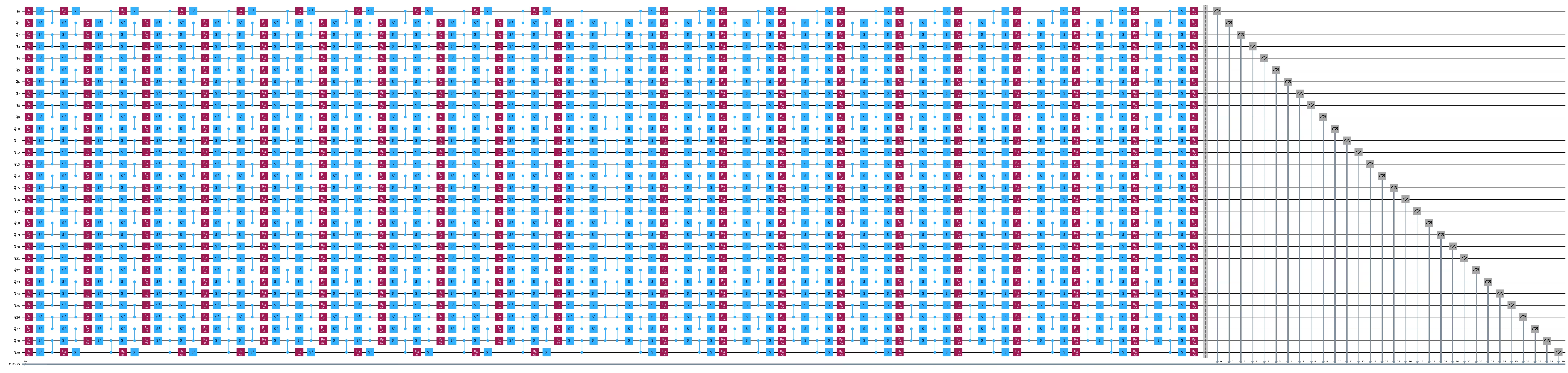
미러링된 트로터 회로와 관측량 생성

이 실험에서는 1차원 스핀 사슬에서 30-사이트 킥드 이징 모델의 시간 역학을 연구합니다. 고려하는 해밀토니안은 다음과 같습니다:

$H = -J\sum\limits_{\langle i,j \rangle} Z_iZ_j + h\sum\limits_iX_i$,

여기서 $J>0$은 최근접 이웃 스핀($i<j$)의 결합을 나타내며, 전역 횡자기장 $h$는 $\frac{\pi}{8}$로 설정됩니다. $h$가 클리퍼드 각도(즉, $\theta=n\frac{\pi}{2}, n \in \mathbb{Z}$)에서 멀어질수록 안티-노이즈 생성자를 회로를 통해 전파하기가 더 어려워집니다.

관측량 선택으로는 평균 단일 사이트 자화, $\frac{1}{N} \sum_{i=1}^{N} \langle z_i \rangle$를 고려합니다. 여기서 $N$은 사이트 수입니다.

num_qubits = 30
num_trotter_steps = 10
rx_angle = np.pi / 8

# Avg single-site magnetization
id_pauli = Pauli("I" * num_qubits)
observable = (
    SparsePauliOp([id_pauli.dot(Pauli("Z"), [i]) for i in range(num_qubits)])
    / num_qubits
)

# Implement Trotterized kicked-Ising model
circuit = QuantumCircuit(num_qubits)
for _step in range(num_trotter_steps):
    circuit.rx(rx_angle, range(num_qubits))
    for first_qubit in (1, 2):
        for idx in range(first_qubit, num_qubits, 2):
            # equivalent to Rzz(-pi/2):
            circuit.sdg([idx - 1, idx])
            circuit.cz(idx - 1, idx)
# Append the inverse circuit to complete the mirroring
circuit.compose(circuit.inverse(), inplace=True)
circuit.measure_active()
circuit.draw("mpl", fold=-1)

2단계: 하드웨어 실행을 위한 문제 최적화

다음 단계는 실제 IBM Quantum 하드웨어에서 실행하기 위해 미러링된 트로터 회로를 준비하는 것입니다. QPU에서 실행하려면 단순히 추상 회로를 구성하는 것 이상의 작업이 필요하며, 다음과 같이 최적화해야 합니다:

1. 백엔드의 네이티브 Gate 세트와 연결성을 준수합니다. 트랜스파일은 논리 회로를 대상 백엔드가 지원하는 ISA 회로로 매핑합니다. 이를 통해 모든 Gate와 Qubit 상호작용이 물리적으로 실현 가능하도록 보장합니다.

2. Circuit 레이어 수준에서 노이즈를 특성화할 수 있습니다. PNA는 역노이즈 채널을 학습하고 전파하는 데 의존합니다. 이를 효율적으로 수행하기 위해, 트랜스파일된 Circuit을 고유한 2-Qubit "박스형" 레이어로 나눕니다. 이러한 박스를 통해 Circuit의 각 레이어를 자체 학습된 노이즈 모델과 연결할 수 있습니다.

3. 현실적인 노이즈 모델을 PNA에 입력할 수 있습니다. Circuit이 박스화되면, NoiseLearnerV3 서비스를 사용하여 각 고유한 2-Qubit 레이어에 영향을 미치는 파울리 노이즈 채널을 실험적으로 학습합니다. 이렇게 학습된 모델은 Samplomatic의 어노테이션을 통해 다시 Circuit에 연결됩니다.

이 단계는 전체적으로 이상화된 미러링된 Circuit과 학습된 노이즈 모델을 갖춘 하드웨어 준비 Circuit 사이의 간극을 메워줍니다. 이 설정을 통해 PNA는 역노이즈 채널을 Circuit을 통해 전파하고 그에 따라 관측량을 조정할 수 있습니다.

백엔드에 연결하고 ISA Circuit으로 트랜스파일

먼저 IBM Quantum Compute Service를 초기화하고 Backend를 선택합니다. 자격 증명을 저장하는 방법에 대한 안내를 따라 사용자 본인의 계정으로 인증하면, 이후 QiskitRuntimeService()가 자동으로 이를 가져옵니다.

# Initialize IBM Quantum Compute Service using your saved credentials
service = QiskitRuntimeService()

backend = service.least_busy(
    operational=True, simulator=False, min_num_qubits=num_qubits
)
# Re-fetch with fractional gates enabled (least_busy does not forward this)
# Fractional gates are enabled so the non-Clifford Rx rotations are supported natively.
backend = service.backend(backend.name, use_fractional_gates=True)
print(f"Selected backend: {backend.name}")

Selected backend: ibm_fez

다음으로, Backend에서 연결된 Qubit 체인을 선택하고 그 위에 Circuit을 트랜스파일합니다.

설정 섹션에서 정의한 find_qubit_chain 헬퍼를 사용하여 연결된 num_qubits개의 물리적 Qubit로 이루어진 라인을 선택합니다. 그런 다음 optimization_level=0으로 트랜스파일하고 이 체인을 initial_layout으로 고정하는데, 이는 미러링된 Circuit의 2-Qubit-Gate 레이어 구조를 정확히 보존합니다. 이 구조는 박스화 및 노이즈 학습 단계가 의존하는 것이므로, 더 높은 최적화 수준(미러링된 Gate를 상쇄할 수 있음)은 여기서 피해야 합니다.

# Find a connected, low-error chain of qubits on the chosen backend
layout = find_qubit_chain(backend, num_qubits)

# Transpile the circuit for the target backend, pinning the chain as the layout.
# optimization_level=0 preserves the mirrored two-qubit-gate layers that the
# boxing and noise-learning steps rely on.
pm = generate_preset_pass_manager(
    backend=backend, optimization_level=0, initial_layout=layout
)
isa_circuit = pm.run(circuit)
isa_observable = observable.apply_layout(isa_circuit.layout)
isa_circuit.draw("mpl", fold=-1)

2-Qubit Gate 레이어와 측정값을 트월링하고 고유한 레이어 찾기

samplomatic을 사용하여 Circuit을 박스화하고 고유한 2-Qubit 레이어를 식별합니다. 박스는 명령어들을 그룹화하여 나중에 동일한 박스 내의 모든 Gate에 특정 의도나 어노테이션을 균일하게 적용할 수 있도록 하는 구조입니다.

여기서는 generate_boxing_pass_manager 메서드를 호출하는데, 이는 단순히 2-Qubit 레이어를 식별하는 것 이상의 작업을 수행합니다. 이 메서드는 다음과 같은 몇 가지 주요 작업을 수행합니다:

• Circuit의 모든 2-Qubit 레이어를 그룹화하고,

• 해당 레이어에 Twirl 및 ChangeBasis 어노테이션을 적용하며,

• 측정 연산을 자체 박스형 섹션으로 그룹화하고,

• 각 2-Qubit 레이어에 InjectNoise 어노테이션을 적용합니다.

이러한 어노테이션은 Circuit 전반에서 노이즈, 기저 변경, 트월링이 처리되는 방식을 정의합니다. 또한 나중에 노이즈를 학습하고 완화하는 데 사용되는 구조를 확립합니다.

주요 구성 옵션은 다음과 같습니다:

• enable_gates/enable_measures: True: 모든 2-Qubit Gate 레이어와 최종 측정을 박스화합니다. 단일 Qubit Gate는 박스 내에서 좌측으로 드레싱됩니다.

• measure_annotations: all: 측정 박스에 Twirl 및 ChangeBasis 어노테이션을 포함합니다.

• twirling_strategy: active: 얽힘 Gate를 포함하는 각 박스에서 모든 활성 Qubit을 트월링합니다.

• inject_noise_targets: gates: 얽힘 Gate를 포함하는 모든 Twirl 어노테이션이 적용된 박스에 InjectNoise 어노테이션을 추가합니다.

• inject_noise_strategy: uniform_modification: Circuit 전체에서 모든 노이즈 레이어를 동일하게 스케일링합니다.

# Box up circuit with Twirl and InjectNoise annotations
pm = generate_boxing_pass_manager(
    enable_gates=True,
    enable_measures=True,
    measure_annotations="all",
    twirling_strategy="active",
    inject_noise_targets="gates",
    inject_noise_strategy="uniform_modification",
)
boxed_circuit = pm.run(isa_circuit)

draw_circ = QuantumCircuit(boxed_circuit.num_qubits)
draw_circ.append(boxed_circuit.data[0], qargs=boxed_circuit.data[0].qubits)
draw_circ.append(boxed_circuit.data[1], qargs=boxed_circuit.data[1].qubits)
draw_circ.draw("mpl", fold=-1, scale=0.3, idle_wires=False)

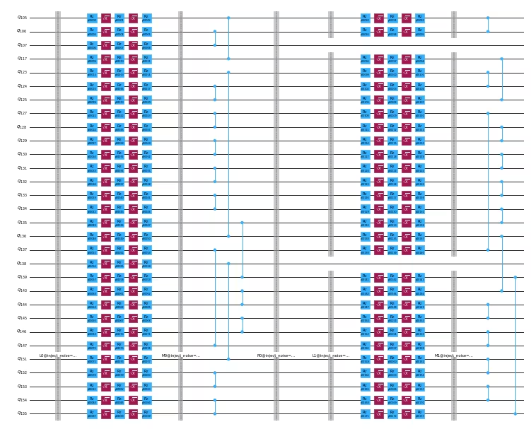
템플릿 Circuit과 Circuit이 샘플링될 방식을 정의하는 samplex를 생성합니다.

여기서는 Executor에서 출력되는 샘플에 대해 후선택을 수행하는 데 필요한 스펙테이터(주변 큐비트) 측정 및 후선택 측정도 추가합니다.

# Build template circuit and samplex for later use with the "Executor"
template_circuit, samplex = samplomatic.build(boxed_circuit)

# Add post-selection instructions to the template circuit
post_selection_pm = PassManager(
    [
        AddSpectatorMeasures(backend.coupling_map),
        AddPostSelectionMeasures(x_pulse_type="rx"),
    ]
)
template_circuit = post_selection_pm.run(template_circuit)

draw_circ = template_circuit.copy_empty_like()
draw_circ.data = template_circuit.data[:324]
draw_circ.draw("mpl", fold=-1, scale=0.3, idle_wires=False)

NoiseLearnerV3를 사용하여 노이즈 학습

오류 완화를 위해 PNA를 적용하기 전에, 먼저 Circuit의 각 고유한 2-Qubit 레이어와 측정 레이어에 작용하는 노이즈를 특성화해야 합니다. 이를 위해 NoiseLearnerV3 프로그램을 사용하여 앞서 식별한 각 레이어에 대한 노이즈 모델을 실험적으로 학습합니다. 이 학습기는 각 레이어에 영향을 미치는 노이즈 채널을 추정하는 벤치마킹 방식의 실험을 수행하고, 학습된 모델을 포함하는 결과 객체를 반환합니다.

먼저 samplomatic의 find_unique_box_instructions를 사용하여 Circuit의 고유한 레이어를 식별합니다. 이렇게 하면 고유한 레이어 유형당 노이즈를 한 번만 학습하게 되어 실험 횟수와 총 샷 비용을 최소화할 수 있습니다. 결과로 나온 레이어 목록은 노이즈 학습기로 전달됩니다.

노이즈가 학습되는 방식을 제어하는 몇 가지 주요 매개변수가 있습니다:

• num_randomizations: 학습 구성당 사용되는 랜덤 Circuit의 수입니다.

• shots_per_randomization: 각 랜덤 학습 Circuit당 취해지는 샷 수입니다.

• layer_pair_depths: 학습 실험에 사용할 Circuit 깊이(쌍의 수로 측정)입니다.

• post_selection: rx Gate를 사용하여 측정 후 펄스를 적용하는 에지 기반 후선택을 활성화합니다.

# Noise learning parameters
num_randomizations_nl = 64
shots_per_randomization_nl = 128

# Match the deepest noise-learning depth to the depth of the circuit being
# mitigated. ``layer_pair_depths`` are measured in layer pairs (a layer + its
# inverse), so the deepest value is half the circuits's two-qubit-layer depth.
# Learning to this depth improves the quality of the mitigation.

depth_2q = isa_circuit.depth(lambda instr: instr.operation.num_qubits == 2)
max_layer_pair_depth = depth_2q // 2

# Use a fixed schedule of learning depths, but drop any that exceed the circuit's
# depth and always cap the deepest value at ``max_layer_pair_depth`` so we never
# learn deeper than the circuit being mitigated
candidate_depths = [1, 2, 4, 8, 12, 16, 24, 32, 40, 48]
layer_pair_depths = sorted(
    {d for d in candidate_depths if d < max_layer_pair_depth}
    | {max_layer_pair_depth}
)

# Find the unique instructions (layers) from the boxed-up circuit
unique_2q_layers_and_meas = find_unique_box_instructions(
    boxed_circuit, normalize_annotations=None, undress_boxes=True
)

# Configure and run the noise learner on the unique layers.
# Options can be passed directly as a dictionary.
noise_learner_options = {
    "num_randomizations": num_randomizations_nl,
    "shots_per_randomization": shots_per_randomization_nl,
    "layer_pair_depths": layer_pair_depths,
    "post_selection": {
        "enable": True,
        "strategy": "edge",
        "x_pulse_type": "rx",
    },
    "environment": {"job_tags": ["TUT_PNA"]},
}

noise_learner = NoiseLearnerV3(backend, noise_learner_options)
noise_learner_job = noise_learner.run(unique_2q_layers_and_meas)
noise_learner_result = noise_learner_job.result()

학습된 노이즈 비율 시각화

노이즈 모델을 학습한 후, 단일 Qubit 연산과 2-Qubit 연산 모두에 대해 추론된 오류율의 분포를 검사할 수 있습니다. 아래 코드는 학습된 노이즈 결과에서 파울리-린드블라드 표현을 추출하고 해당 노이즈 비율을 수집합니다.

학습된 각 레이어에 대해:

• 노이즈 모델을 (pstr, qubits, rate) 튜플의 희소 목록으로 변환합니다. 여기서 pstr은 주어진 Qubit에 작용하는 파울리 문자열이고 rate는 관련된 오류율입니다.
• 비율을 단일 Qubit(len(pstr) == 1) 항과 2-Qubit(len(pstr) == 2) 항으로 분리합니다.
• 비율 목록을 정렬한 다음 중앙값을 계산합니다.

학습된 파울리-린드블라드 생성자의 상대적 크기를 비교할 수 있도록, 단일 Qubit(빨간색)과 2-Qubit(파란색) 노이즈 비율 분포를 로그 스케일로 그리고, 중앙값을 수직선으로 표시합니다. 단일 Qubit 비율과 2-Qubit 비율의 순서는 장치와 특성화되는 특정 레이어에 따라 달라지며, 이번 실행에서는 단일 Qubit(가중치 1) 생성자가 더 큰 중앙값을 갖습니다.

hw_rates_1q = []
hw_rates_2q = []
for nlr in noise_learner_result[:2]:
    plm_list = nlr.to_pauli_lindblad_map().to_sparse_list()
    hw_rates_1q += [
        rate for (pstr, qubits, rate) in plm_list if len(pstr) == 1
    ]
    hw_rates_2q += [
        rate for (pstr, qubits, rate) in plm_list if len(pstr) == 2
    ]
hw_rates_1q = sorted(hw_rates_1q)
hw_rates_2q = sorted(hw_rates_2q)
median_1q = hw_rates_1q[len(hw_rates_1q) // 2]
median_2q = hw_rates_2q[len(hw_rates_2q) // 2]
fig, ax = plt.subplots(1, 1, figsize=(14, 5))
ax.scatter(
    (hw_rates_1q),
    [(i) / (len(hw_rates_1q) - 1) for i in range(len(hw_rates_1q))],
    color="red",
    label="1q rates",
)
ax.set_xscale("log")
ax.set_ylim(0, 1.1)
ax.vlines(median_1q, 0, 1, color="red")
ax.text(median_1q * 1.1, 0.1, f"{median_1q:.2e}")
ax.scatter(
    (hw_rates_2q),
    [(i) / (len(hw_rates_2q) - 1) for i in range(len(hw_rates_2q))],
    color="blue",
    label="2q rates",
)
ax.set_xscale("log")
ax.set_ylim(0, 1.1)
ax.vlines(median_2q, 0, 1, color="blue")
ax.text(median_2q * 1.1, 0.2, f"{median_2q:.2e}")
ax.set_title("Learned noise rates")
ax.set_xlabel("Noise rate")
ax.set_yticks([])
plt.legend()

<matplotlib.legend.Legend at 0x125336120>

Circuit 박스를 학습된 노이즈와 연결

각 고유한 2-Qubit 레이어에 대한 노이즈 모델을 얻은 후, 이를 박스화된 Circuit 내의 해당 InjectNoise 어노테이션과 연결해야 합니다.

InjectNoise 지시어는 단일 Qubit 드레서를 사용하여 제어되고 구성 가능한 방식으로 Circuit에 노이즈를 주입하는 samplomatic 어노테이션입니다. 이를 통해 서로 다른 레이어 간의 모듈식 노이즈 모델링이 가능합니다.

각 InjectNoise 어노테이션은 다음을 포함합니다:

• InjectNoise.ref - 어노테이션에 대한 고유 식별자입니다. samplex 객체가 이를 사용하여 해당 노이즈 모델을 올바르게 할당합니다.
• InjectNoise.modifier_ref (선택 사항) - 할당된 노이즈 모델을 곱셈 계수로 스케일링할 수 있게 해주는 보조 참조입니다.

이 단계에서는 각 InjectNoise.ref를 해당 학습된 노이즈 모델(PauliLindbladMap)에 대응시키는 매핑을 구성합니다. 이 매핑을 통해 Circuit의 각 얽힘 Gate 레이어가 적절한 노이즈 모델과 짝지어져, 샘플링 및 이후 노이즈 완화 단계에서 노이즈 영향이 정확하게 적용되도록 합니다.

# map inject noise refs to pauli lindblad maps
refs_to_noise_models = {}
for instruction, result in zip(
    unique_2q_layers_and_meas, noise_learner_result, strict=False
):
    if inject_noise_annot := get_annotation(
        instruction.operation, InjectNoise
    ):
        refs_to_noise_models[inject_noise_annot.ref] = (
            result.to_pauli_lindblad_map()
        )

학습된 안티-노이즈를 통해 관측량 전파

위에서 설명했듯이, 이는 두 단계로 이루어집니다. 먼저 안티-노이즈 생성자를 Circuit 끝까지 전파합니다. 그런 다음 관측량을 그 진화된 생성자를 통해 전파합니다. 이 과정은 Circuit의 각 안티-노이즈 생성자에 대해 반복됩니다. 이 구현에서는 주어진 레이어의 각 생성자가 병렬로 Circuit 끝까지 전파됩니다. 또한 Python 멀티프로세싱을 사용하여 안티-노이즈의 순방향 전파와 관측량의 역방향 전파를 모두 병렬로 수행합니다. 이렇게 하면 메모리에 진화된 생성자가 쌓이는 것을 방지하고 컴퓨팅 리소스를 최대한 활용할 수 있습니다.

PNA를 실행할 때는 항상 노이즈가 있는 Circuit과 관측량을 제공해야 합니다. 노이즈가 있는 Circuit이 InjectNoise 어노테이션이 있는 박스형 Circuit인 경우, 위 단계에서 생성한 매핑을 제공해야 합니다. qiskit-aer의 PauliLindbladError 명령어를 포함하는 박스화되지 않은 Circuit을 전달할 수도 있습니다. 이 경우 refs_to_noise_models를 제공할 필요가 없습니다. 기본 입력 외에도 다음 사항을 고려하세요:

• max_err_terms: 순방향 전파될 때 각 안티-노이즈 생성자에 유지할 항의 수입니다. 이 값을 크게 허용하면 일반적으로 정확도가 향상되지만, 이 동작이 단조롭다고 보장되지는 않습니다.

• max_obs_terms: 진화된 안티-노이즈를 통해 역방향 전파될 때 노이즈 완화 관측량 $\tilde{O}$에 유지할 항의 수입니다. 값이 클수록 일반적으로 정확도가 향상되지만, 이것이 단조롭게 보장되지는 않습니다.

• num_processes: 이 프로세스에 할당할 코어 수입니다. 생성자는 순방향으로 전파되고 관측량에 병렬로 적용된다는 점을 기억하세요.

• search_step: 역방향 전파 단계는 그리디 방법을 사용하여 파울리 기저에서 두 연산자를 근사적으로 켤레화합니다. 이 방법은 search_step을 늘려서 속도를 높일 수 있습니다. 자세한 내용은 pauli-prop 문서를 참조하세요.

• num_to_measure: 이 변수는 generate_noise_mitigating_observable의 입력은 아니지만, $\tilde{O}$에서 실제로 측정하고자 하는 항의 수를 제어하는 데 사용합니다. 여기서는 원래 관측량의 원래 항인 상위 30개 항만 측정합니다. 이 항들은 이제 측정 시 학습된 Gate 노이즈를 완화하는 효과가 있도록 재조정되었습니다. $\tilde{O}$에서 30개 항만 측정하지만, 이를 크게 성장시키는 것이 여전히 유용한 경우가 많은데, 이는 선도 항들의 스케일링 계수의 정밀도를 높이기 때문입니다.

# PNA parameters
num_processes = 8
max_err_terms = 10_000
max_obs_terms = 10_000
num_to_measure = num_qubits

obs_tilde_isa = generate_noise_mitigating_observable(
    boxed_circuit,
    isa_observable,
    refs_to_noise_models,
    max_err_terms=max_err_terms,
    max_obs_terms=max_obs_terms,
    num_processes=num_processes,
    print_progress=True,
    search_step=8,
)
p_2_v = {p: v for v, p in enumerate(layout)}
obs_tilde_virtual = SparsePauliOp.from_sparse_list(
    [
        (pstr, [p_2_v[p] for p in p_qubits], coeff)
        for (pstr, p_qubits, coeff) in obs_tilde_isa.to_sparse_list()
    ],
    num_qubits=num_qubits,
)
obs_tilde_virtual = obs_tilde_virtual[
    np.argsort(np.abs(obs_tilde_virtual.coeffs))[::-1]
][:num_to_measure]

Finished! 13740 / 13740 generators propagated.

obs_tilde_isa = obs_tilde_isa[np.argsort(np.abs(obs_tilde_isa.coeffs))][::-1]
plt.xscale("log")
plt.yscale("log")
plt.title(r"$\tilde{O}$ coeff magnitudes")
plt.ylabel("Magnitude")
plt.xlabel("Pauli term index")
plt.plot(np.abs(obs_tilde_isa.coeffs), ".")

[<matplotlib.lines.Line2D at 0x124b0a120>]

측정 기저를 표준형으로 변환

다음으로, 측정된 관측량의 모든 파울리 항을 완전히 포괄할 수 있는 측정할 기저의 최소 집합을 찾습니다(여러 관측량이 큐빗별로 교환 가능하다면 동시에 측정될 수 있습니다). 원래 관측량의 항만 측정하고 있으며 이는 모든 단일-Z 파울리의 합이므로, 하나의 기저만 필요합니다: 전체-Z 기저입니다.

파울리 측정 기저 집합을 찾는 것 외에도, 이러한 파울리 항을 Executor가 기대하는 표준형으로 매핑해야 합니다. 표준 Qubit 순서에 대한 자세한 내용은 Samplomatic 문서를 참조하세요.

meas_box = boxed_circuit.data[-1]
canonical_qubits = [
    idx
    for idx, qubit in enumerate(boxed_circuit.qubits)
    if qubit in meas_box.qubits
]
c_2_p = {
    c: p for c, p in enumerate(canonical_qubits)
}  # canonical -> physical
p_2_v = {p: v for v, p in enumerate(layout)}  # physical -> virtual
c_2_v = {c: p_2_v[p] for c, p in c_2_p.items()}  # canonical -> virtual
meas_bases, bases_reverser = get_measurement_bases(obs_tilde_virtual)
meas_bases_canonical = [
    np.array([base[c_2_v[c]] for c in range(num_qubits)], dtype=np.uint8)
    for base in meas_bases
]

3단계: 양자 실험 실행

QuantumProgram에서 샘플링 방법 지정

이제 Executor에 의해 실행될 모든 Circuit과 샘플링 구성의 중앙 컨테이너 역할을 하는 QuantumProgram을 설정합니다. 이 객체는 PNA에 사용되는 측정 결과를 생성하기 위해 무작위화된 Circuit 인스턴스가 생성, 배치 및 실행되는 방식을 정의합니다.

QuantumProgram은 각각 템플릿 Circuit과 무작위화가 적용되는 방식을 정의하는 해당 samplex 객체로 구성된 여러 항목을 포함할 수 있습니다. 이 추상화를 통해 Executor는 무작위화된 Circuit 생성부터 샷 수집 및 집계에 이르는 전체 워크플로우를 하나의 모듈식 프로그램으로 처리할 수 있습니다.

이 단계에서는 앞서 구성한 템플릿 Circuit과 samplex를 사용하여 PNA 실험을 실행하는 QuantumProgram을 생성합니다. 이 구성에는 다음 요소가 포함됩니다:

• template_circuit: 원하는 모든 랜덤화(트월링 랜덤화, 매개변수 등)를 구현하는 데 필요한 모든 Gate를 포함하는 Circuit입니다.

• samplex: 샘플링할 수 있는 가능한 모든 Circuit 랜덤화에 대한 확률 분포를 정의하는 객체입니다.

• samplex_arguments: samplex를 완전히 정의하는 데 필요한 바인딩입니다

  • basis_changes: 여기서 측정된 관측량의 모든 파울리 항을 포괄할 측정 기저 집합을 지정합니다.

  • noise_scales.ref: 샘플에 추가 노이즈가 주입되지 않도록 각 노이즈 레이어의 스케일을 0.0으로 설정합니다.

  • pauli_lindblad_maps: noise_scales가 전달되는 경우 필수입니다. 이는 노이즈 레이어를 관련된 노이즈 모델에 매핑합니다.

• shape: samplex_arguments에 의해 정의된 암시적 형태를 확장하는 형태 튜플입니다. 이 확장으로 도입된 비자명 축은 랜덤화를 열거합니다.

# Control the # of shots during execution
shots_per_randomization_exec = 64
num_randomizations_exec = 6144

# Zero out the noise to prevent noise from being injected during execution.
# We only added InjectNoise annotations so PNA could associate the noise
# to layers in the circuit
samplex_inputs = {f"noise_scales.{ref}": 0.0 for ref in refs_to_noise_models}
samplex_inputs |= {"pauli_lindblad_maps": refs_to_noise_models}

# Specify the bases to measure. The samplex exposes one basis-change input per
# ChangeBasis-annotated box; here a single all-Z basis covers every term. We
# look up the basis-change interface name rather than hardcoding an index, since
# the name depends on the circuit's box structure.
bases_broadcastable = np.expand_dims(np.array(meas_bases_canonical), axis=1)
samplex_inputs |= {
    spec.name: bases_broadcastable
    for spec in samplex.inputs().get_specs(r"^basis_changes\.")
}

# Convert samplex_inputs into a dict to pass to QuantumProgram
samplex_arguments = (
    samplex.inputs().make_broadcastable().bind(**samplex_inputs)
)

# Instantiate the QuantumProgram with the specified parameters
program = QuantumProgram(shots=shots_per_randomization_exec)
program.append_samplex_item(
    circuit=template_circuit,
    samplex=samplex,
    samplex_arguments=samplex_arguments,
    shape=(num_randomizations_exec,),
)

Executor를 사용하여 Circuit 샘플링

QuantumProgram을 정의했으므로, 실험을 실행하는 것은 간단합니다. Executor 객체를 인스턴스화하고, Backend를 제공한 다음, 프로그램을 실행하기만 하면 됩니다.

# Execute (sample) the circuit
executor = Executor(backend)
job_exec = executor.run(program)
exec_results = job_exec.result()

4단계: 결과 재구성 및 분석

오류 완화된 기댓값을 계산하기 위해 다음을 수행합니다:

• 측정에 영향을 미치는 학습된 노이즈를 기반으로 TREX 스케일링 계수를 계산하고,

• 후선택된 샘플만 유지하기 위한 마스크를 생성하며,

• qiskit-addon-utils의 executor_expectation_values 함수를 사용하여 모든 데이터를 오류 완화된 기댓값으로 결합합니다.

# Computing the TREX factors
measurement_noise_map = noise_learner_result[2].to_pauli_lindblad_map()
trex_rescale_factors = trex_factors(measurement_noise_map, bases_reverser)

# Post-select the results
post_selector = PostSelector.from_circuit(
    circuit=template_circuit, coupling_map=backend.coupling_map
)

# Compute the ps mask for filtering results
mask = post_selector.compute_mask(exec_results[0], strategy="edge")

# Compute expvals using post selected results
results = executor_expectation_values(
    exec_results[0]["meas"],
    bases_reverser,
    meas_basis_axis=0,
    avg_axis=1,
    measurement_flips=exec_results[0]["measurement_flips.meas"],
    pauli_signs=exec_results[0].get("pauli_signs", None),
    postselect_mask=mask,
    rescale_factors=trex_rescale_factors,
)

완화 전략 비교: PNA, PNA+TREX, PNA+PS, PNA+PS+TREX

Executor 결과를 사용하여 여러 완화 변형에 대한 기댓값을 계산하고 시각화합니다.

bases_reverser_unmit = {Pauli("Z" * num_qubits): [observable]}
args = [
    (bases_reverser_unmit, None, None),
    (bases_reverser, None, None),
    (bases_reverser, None, trex_rescale_factors),
    (bases_reverser, mask, None),
    (bases_reverser, mask, trex_rescale_factors),
]

evs = []
for reverser, postsel_mask, factors in args:
    # Compute expvals using post selected results
    res_ps = executor_expectation_values(
        exec_results[0]["meas"],
        reverser,
        meas_basis_axis=0,
        avg_axis=1,
        measurement_flips=exec_results[0]["measurement_flips.meas"],
        pauli_signs=exec_results[0].get("pauli_signs", None),
        postselect_mask=postsel_mask,
        rescale_factors=factors,
    )
    res_ps = np.array(res_ps)
    evs.append(res_ps[:, 0][0])

experiments = ["PNA", "PNA+TREX", "PNA+PS", "PNA+PS+TREX"]
colors = ["#d9d9d9", "#b0b0b0", "#7f7f7f", "#4c4c4c"]
plt.bar(experiments, evs[1:], color=colors)
plt.axhline(y=1, color="green", linestyle="--", linewidth=2, label="Ideal")
plt.axhline(
    y=evs[0], color="red", linestyle="--", linewidth=2, label="Unmitigated"
)
plt.ylabel("Expectation value", fontsize=14)

plt.title(
    r"30q Mirrored Ising, 10 Trotter steps, $\theta_{rx}=\frac{\pi}{8}$",
    fontsize=14,
)
plt.legend(loc="upper left", bbox_to_anchor=(1.05, 1), borderaxespad=0.0)
plt.xticks(rotation=45)
plt.tight_layout()
plt.show()

이 결과는 서로 다른 오류 완화 기법을 결합했을 때의 누적 이점을 보여줍니다. 순수한 PNA 접근법만으로도 이미 기댓값을 이상적인 벤치마크에 가깝게 복원하며, 이는 역노이즈 채널을 관측량에 전파하는 것이 2-Qubit Gate 오류를 효과적으로 보상함을 나타냅니다.

• TREX 재가중치(PNA+TREX)를 추가하면 랜덤화된 Circuit의 샘플링 불균형을 보정하여 추정값을 약간 개선합니다.

• 후선택(PNA+PS)은 잔여 오류로 인해 발생할 가능성이 높은 일관되지 않은 측정 결과를 걸러내어 더 눈에 띄는 향상을 제공합니다.

• 마지막으로, 둘 다 결합하면(PNA+PS+TREX) 가장 정확한 결과를 얻으며, 이상적인 값과 거의 일치하여 이러한 완화 전략들이 서로를 강화함을 보여줍니다.

전반적으로, 이 비교는 PNA가 노이즈를 인식하는 기댓값 추정을 위한 견고한 기반 역할을 하는 반면, TREX와 후선택은 추가적인 정확도 향상을 위한 상호 보완적인 개선을 제공한다는 점을 강조합니다.

다음 단계

이 작업에 관심이 있으시다면, 다음 자료에도 관심을 가지실 수 있습니다:

Recommendations

• Estimator 프리미티브와 오류 완화 옵션 결합
• 확률적 오류 증폭을 활용한 유틸리티 규모 오류 완화
• 기댓값 추정을 위한 연산자 역전파(OBP)
• samplomatic 및 pauli-prop 문서