Qiskit AI 기반 Transpiler 소개

예상 사용 시간: IBM Heron에서 5분 (참고: 이는 예상치이며 실제 실행 시간은 다를 수 있습니다.)

학습 목표

이 튜토리얼을 마치면 사용자는 다음을 이해할 수 있습니다:

• AI 기반 Transpiler(generate_ai_pass_manager)를 표준 Transpiler의 대체품으로 사용하는 방법
• AI 기반 Transpiler가 두 Qubit 깊이, Gate 수, 트랜스파일 시간 측면에서 기본 Transpiler와 어떻게 비교되는지
• 미러 Circuit을 사용하여 하드웨어 실행을 통해 트랜스파일 품질을 평가하는 방법

사전 요구 사항

이 튜토리얼을 진행하기 전에 다음 주제에 대해 잘 알고 있는 것이 좋습니다:

• Circuit 트랜스파일
• 프리셋 패스 매니저 구성
• AI 기반 Transpiler 패스

배경

Qiskit AI 기반 Transpiler는 SABRE와 같은 전통적인 휴리스틱 방법보다 더 짧고 하드웨어 효율적인 Circuit을 생성할 수 있는 머신 러닝 기반 트랜스파일 패스를 도입합니다. 더 짧은 Circuit은 노이즈를 덜 축적하여 실제 양자 하드웨어에서 결과 품질을 직접적으로 향상시킵니다.

이 튜토리얼에서는 두 가지 트랜스파일 전략을 비교합니다:

전략	API
기본	generate_preset_pass_manager(optimization_level=3, ...)
AI	generate_ai_pass_manager(optimization_level=1, ai_optimization_level=3, ...)

각 전략에 대해 세 가지 지표를 측정합니다: 두 Qubit Gate 깊이, 총 Gate 수, 트랜스파일 런타임.

AI 기반 Transpiler 벤치마크

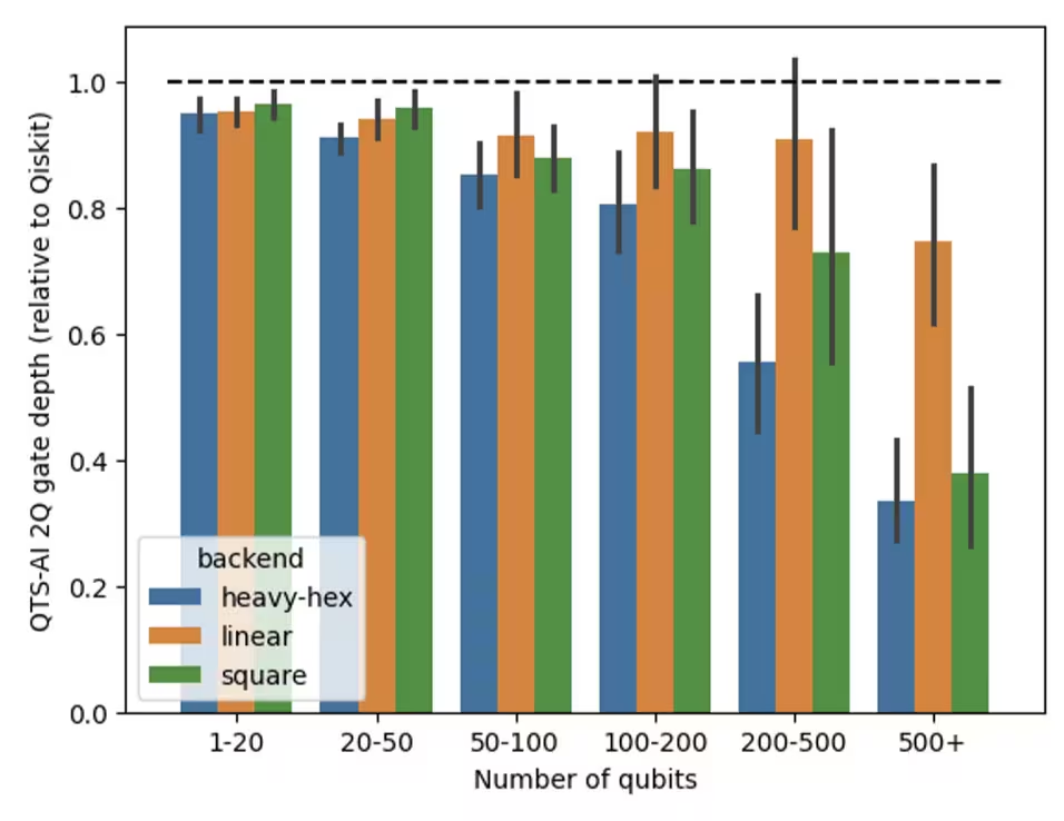
벤치마킹 테스트에서 AI 기반 Transpiler는 표준 Qiskit Transpiler에 비해 일관되게 더 얕고 품질이 높은 Circuit을 생성했습니다. 이 테스트에서는 generate_preset_pass_manager로 구성된 Qiskit의 기본 패스 매니저 전략을 사용했습니다. 이 기본 전략은 종종 효과적이지만 더 크거나 복잡한 Circuit에서는 어려움을 겪을 수 있습니다. 반면에 AI 기반 패스는 IBM Quantum® 하드웨어의 heavy-hex 토폴로지로 트랜스파일할 때 대규모 Circuit(100개 이상의 Qubit)에서 평균 24%의 두 Qubit Gate 수 감소와 36%의 Circuit 깊이 감소를 달성했습니다. 이 벤치마크에 대한 자세한 내용은 이 블로그를 참고하세요.

이 튜토리얼은 AI 패스의 주요 이점과 기존 방법과의 비교를 살펴봅니다.

요구 사항

이 튜토리얼을 시작하기 전에 다음이 설치되어 있는지 확인하세요:

• 시각화 지원이 포함된 Qiskit SDK v2.0 이상
• Qiskit Runtime (pip install qiskit-ibm-runtime) v0.22 이상
• AI 로컬 모드가 포함된 Qiskit IBM Transpiler (pip install 'qiskit-ibm-transpiler[ai-local-mode]')
• Qiskit Aer (pip install qiskit-aer)

설정

# Added by doQumentation — required packages for this notebook
!pip install -q matplotlib qiskit qiskit-aer qiskit-ibm-runtime qiskit-ibm-transpiler

from qiskit import QuantumCircuit
from qiskit.circuit.random import random_circuit
from qiskit.transpiler import generate_preset_pass_manager
from qiskit_ibm_runtime import QiskitRuntimeService, SamplerV2
from qiskit_ibm_transpiler import generate_ai_pass_manager
from qiskit_aer import AerSimulator
from qiskit_aer.noise import NoiseModel, depolarizing_error
import matplotlib.pyplot as plt
from statistics import mean, stdev
import time
import logging

seed = 42

def transpile_with_metrics(pass_manager, circuit):
    """Transpile a circuit and return the result along with key metrics."""
    start = time.time()
    qc_out = pass_manager.run(circuit)
    elapsed = time.time() - start

    depth_2q = qc_out.depth(lambda x: x.operation.num_qubits == 2)
    gate_count = qc_out.size()

    return qc_out, {
        "depth_2q": depth_2q,
        "gate_count": gate_count,
        "time_s": round(elapsed, 3),
    }

def remap_to_contiguous(tqc):
    """Remap a transpiled circuit to use contiguous qubit indices.

    Transpiled circuits target specific physical qubits (e.g., qubit 45, 67)
    on a large backend. This remaps them to 0, 1, 2, ... so Aer only
    simulates the active qubits."""
    active = sorted(
        {tqc.find_bit(q).index for inst in tqc.data for q in inst.qubits}
    )
    qubit_map = {old: new for new, old in enumerate(active)}
    new_qc = QuantumCircuit(len(active))
    for inst in tqc.data:
        old_indices = [tqc.find_bit(q).index for q in inst.qubits]
        new_qc.append(inst.operation, [qubit_map[i] for i in old_indices])
    return new_qc

def build_mirror_circuit(tqc, simulate=True):
    """Build a mirror circuit: U followed by U-dagger, with measurements.

    The expected output is always |0...0>, so measuring the survival
    probability reveals how much noise each transpilation strategy adds.

    Args:
        tqc: A transpiled circuit.
        simulate: If True (default), remap to contiguous qubits so Aer
            only simulates the active qubits. If False, keep the full
            physical layout for hardware execution."""
    if simulate:
        tqc = remap_to_contiguous(tqc)
    mirror = tqc.compose(tqc.inverse())
    mirror.measure_all()
    return mirror

def print_summary(results):
    """Print a summary of each metric as mean +/- stdev across all circuits,
    along with the mean percentage improvement of AI over Default."""
    metrics = [
        ("Depth 2Q", "Depth 2Q (Default)", "Depth 2Q (AI)"),
        ("Gate Count", "Gate Count (Default)", "Gate Count (AI)"),
        ("Time (s)", "Time (Default)", "Time (AI)"),
    ]
    header = (
        f"{'Metric':<12}{'Default (mean +/- std)':>24}"
        f"{'AI (mean +/- std)':>22}{'AI % improvement':>22}"
    )
    print(header)
    print("-" * len(header))
    for label, col_def, col_ai in metrics:
        defaults = [r[col_def] for r in results]
        ais = [r[col_ai] for r in results]
        pct = [(d - a) / d * 100 for d, a in zip(defaults, ais)]
        default_str = f"{mean(defaults):.1f} +/- {stdev(defaults):.1f}"
        ai_str = f"{mean(ais):.1f} +/- {stdev(ais):.1f}"
        pct_str = f"{mean(pct):+.1f}% +/- {stdev(pct):.1f}%"
        print(f"{label:<12}{default_str:>24}{ai_str:>22}{pct_str:>22}")

def plot_metrics_and_pct(results, title_prefix):
    """Plot metric comparisons and percentage improvement of AI over Default."""
    qubits = [r["Qubits"] for r in results]
    metrics = [
        ("Depth 2Q (Default)", "Depth 2Q (AI)", "Two-Qubit Depth"),
        ("Gate Count (Default)", "Gate Count (AI)", "Gate Count"),
        ("Time (Default)", "Time (AI)", "Transpilation Time"),
    ]

    # Row 1: raw metric comparison
    fig, axs = plt.subplots(1, 3, figsize=(21, 5))
    fig.suptitle(
        f"{title_prefix}: Metric Comparison",
        fontsize=15,
        fontweight="bold",
        y=1.02,
    )
    for ax, (col_def, col_ai, label) in zip(axs, metrics):
        ax.plot(qubits, [r[col_def] for r in results], "o-", label="Default")
        ax.plot(qubits, [r[col_ai] for r in results], "s-", label="AI")
        ax.set_title(label)
        ax.set_xlabel("Number of Qubits")
        ax.set_ylabel(label)
        ax.legend()
    plt.tight_layout()
    plt.show()

    # Row 2: percentage improvement
    fig, axs = plt.subplots(1, 3, figsize=(21, 5))
    fig.suptitle(
        f"{title_prefix}: % Improvement of AI over Default",
        fontsize=15,
        fontweight="bold",
        y=1.02,
    )
    for ax, (col_def, col_ai, label) in zip(axs, metrics):
        pct = [(r[col_def] - r[col_ai]) / r[col_def] * 100 for r in results]
        ax.axhline(
            0, color="#1f77b4", linewidth=2, label="Default (baseline)"
        )
        ax.plot(qubits, pct, "s-", color="#ff7f0e", label="AI")
        ax.fill_between(qubits, 0, pct, alpha=0.15, color="#ff7f0e")
        ax.set_title(label)
        ax.set_xlabel("Number of Qubits")
        ax.set_ylabel("% Improvement")
        ax.legend()
    plt.tight_layout()
    plt.show()

# Suppress verbose AI-powered transpiler logs
logging.getLogger(
    "qiskit_ibm_transpiler.wrappers.ai_local_synthesis"
).setLevel(logging.WARNING)

소규모 시뮬레이터 예제

Step 1: 고전적 입력을 양자 문제로 매핑

깊이 4의 무작위 Circuit 20개를 생성합니다. Qubit 수는 6개에서 25개까지 범위입니다. 이 Circuit들은 트랜스파일 전략을 비교하기 위한 테스트 케이스로 사용됩니다.

num_circuits_sim = 20
depth_sim = 4
qubit_range_sim = list(range(6, 26))

circuits_sim = [
    # We have only two qubit gates, as those test how well the transpiler can optimize the circuit.
    random_circuit(
        num_qubits=n,
        depth=depth_sim,
        max_operands=2,
        num_operand_distribution={2: 1},
        seed=seed + i,
    )
    for i, n in enumerate(qubit_range_sim)
]

print(
    f"Created {len(circuits_sim)} circuits with qubit counts: {qubit_range_sim}"
)
circuits_sim[0].draw(output="mpl", fold=-1)

Created 20 circuits with qubit counts: [6, 7, 8, 9, 10, 11, 12, 13, 14, 15, 16, 17, 18, 19, 20, 21, 22, 23, 24, 25]

Step 2: 양자 하드웨어 실행을 위한 문제 최적화

선택한 Backend에 대해 기본(SABRE) 패스 매니저를 구성합니다. 두 트랜스파일 전략 모두 Backend의 전체 커플링 맵을 대상으로 합니다. 시뮬레이션 단계에서는 remap_to_contiguous를 사용하여 각 트랜스파일된 Circuit을 활성 Qubit에만 다시 레이블링하므로, Aer는 전체 디바이스 대신 해당 Qubit만 시뮬레이션합니다.

service = QiskitRuntimeService()
backend = service.least_busy(
    min_num_qubits=100, operational=True, simulator=False
)

pm_default_sim = generate_preset_pass_manager(
    optimization_level=3,
    backend=backend,
    seed_transpiler=seed,
)

results_sim = []

for i, qc in enumerate(circuits_sim):
    n = qubit_range_sim[i]

    qc_default, m_default = transpile_with_metrics(pm_default_sim, qc)

    # Create a fresh AI pass manager each iteration to avoid stale layout state
    pm_ai = generate_ai_pass_manager(
        optimization_level=1,
        ai_optimization_level=3,
        backend=backend,
    )
    qc_ai, m_ai = transpile_with_metrics(pm_ai, qc)

    results_sim.append(
        {
            "Qubits": n,
            "Depth 2Q (Default)": m_default["depth_2q"],
            "Depth 2Q (AI)": m_ai["depth_2q"],
            "Gate Count (Default)": m_default["gate_count"],
            "Gate Count (AI)": m_ai["gate_count"],
            "Time (Default)": m_default["time_s"],
            "Time (AI)": m_ai["time_s"],
        }
    )

print_summary(results_sim)

Fetching 4 files:   0%|          | 0/4 [00:00<?, ?it/s]

Metric        Default (mean +/- std)     AI (mean +/- std)      AI % improvement
--------------------------------------------------------------------------------
Depth 2Q               33.0 +/- 12.9          26.4 +/- 8.0      +15.8% +/- 17.6%
Gate Count           522.0 +/- 266.0       560.5 +/- 279.1        -9.0% +/- 9.0%
Time (s)                 0.0 +/- 0.0           0.2 +/- 0.1    -893.6% +/- 362.9%

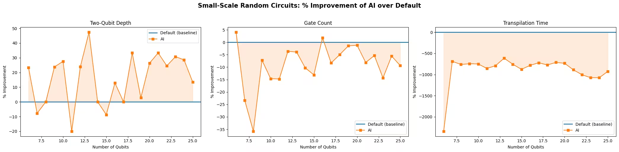
요약 표는 20개의 Circuit 전체에 걸친 각 지표의 평균 및 표준 편차와 기본 대비 AI 기반 Transpiler의 평균 개선율을 보여줍니다. 양수 값은 AI 기반 Transpiler가 더 나은 결과를 냈음을, 음수 값은 기본값이 더 나았음을 나타냅니다.

이 소규모 예제에서 AI 기반 Transpiler는 평균적으로 약 16% 낮은 두 Qubit 깊이를 달성하지만, 약 9% 더 높은 Gate 수를 희생합니다. 이는 두 전략 중 선택할 때의 주요 절충점을 강조합니다: AI 기반 Transpiler는 깊이 감소(더 적은 두 Qubit Gate의 순차적 레이어)를 우선시하는 반면, 기본 Transpiler(SABRE)는 총 Gate 수 최소화(더 적은 SWAP 삽입)를 우선시합니다. 애플리케이션에 따라 한 지표가 다른 지표보다 더 중요할 수 있습니다.

plot_metrics_and_pct(results_sim, "Small-Scale Random Circuits")

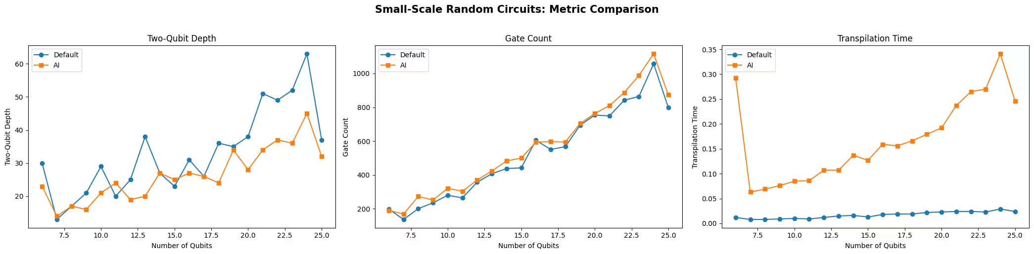
두 Qubit 깊이: AI 기반 Transpiler는 일반적으로 더 낮은 두 Qubit 깊이를 가진 Circuit을 생성합니다. 깊이는 AI 라우팅 모델이 최적화하도록 훈련된 주요 지표 중 하나이며, 대부분의 Circuit 크기에서 개선이 보이지만 개별 Circuit에서는 SABRE가 동일하거나 더 나은 결과를 낼 수도 있습니다.

Gate 수: 이 규모에서 결과가 비슷하게 나타나며, SABRE가 전반적으로 약간의 우위를 유지합니다. SABRE의 라우팅 휴리스틱은 삽입되는 SWAP Gate 수를 최소화하도록 설계되어 있어 Gate 수를 직접적으로 줄입니다. 소규모 Circuit 크기에서는 차이가 적습니다.

트랜스파일 시간: SABRE의 런타임은 Qubit 수에 관계없이 거의 일정하므로 Circuit 크기가 이 규모에서 트랜스파일 시간에 거의 영향을 미치지 않습니다. SABRE의 핵심 라우팅 로직은 고도로 최적화되어 있습니다(주로 Rust로 구현됨). AI 기반 Transpiler는 눈에 띄게 더 오래 걸리고 Circuit 크기에 따라 확장되지만, 절대 시간은 대화형 사용에 합리적인 수준을 유지합니다.

Step 3: Qiskit 프리미티브를 사용한 실행

트랜스파일이 Circuit 충실도에 미치는 영향을 평가하기 위해 10-Qubit 케이스에서 미러 Circuit을 구성하고 간단한 노이즈 모델이 적용된 Aer 시뮬레이터에서 실행합니다. 미러 Circuit의 예상 출력은 항상 모두 0인 비트스트링이므로, $|0\rangle^{\otimes n}$을 측정할 확률은 각 트랜스파일 전략이 충실도를 얼마나 잘 유지하는지 보여줍니다.

# Use the 10-qubit circuit (index where qubits == 10)
idx_10q = qubit_range_sim.index(10)

qc_10q = circuits_sim[idx_10q]
qc_default_10q, _ = transpile_with_metrics(pm_default_sim, qc_10q)

pm_ai = generate_ai_pass_manager(
    optimization_level=1,
    ai_optimization_level=3,
    backend=backend,
)
qc_ai_10q, _ = transpile_with_metrics(pm_ai, qc_10q)

tqc_methods = {
    "Default": qc_default_10q,
    "AI": qc_ai_10q,
}

print(
    f"Default: depth {qc_default_10q.depth()}, gates {qc_default_10q.size()}"
)
print(f"AI:      depth {qc_ai_10q.depth()}, gates {qc_ai_10q.size()}")

Default: depth 84, gates 280
AI:      depth 91, gates 343

# Build a simple depolarizing noise model
noise_model = NoiseModel()
noise_model.add_all_qubit_quantum_error(
    depolarizing_error(0.001, 1),
    ["sx", "x", "rz"],  # ~0.1% per 1Q gate
)
noise_model.add_all_qubit_quantum_error(
    depolarizing_error(0.01, 2),
    ["cx", "ecr"],  # ~1% per 2Q gate
)

aer_sim = AerSimulator(noise_model=noise_model)

shots = 10000
survival_probs = {}

for method, tqc in tqc_methods.items():
    mirror = build_mirror_circuit(tqc, simulate=True)

    sampler = SamplerV2(mode=aer_sim)
    job = sampler.run([mirror], shots=shots)
    counts = job.result()[0].data.meas.get_counts()

    all_zeros = "0" * mirror.num_qubits
    survival = counts.get(all_zeros, 0) / shots
    survival_probs[method] = survival
    print(
        f"{method:8s}  P(|00...0>) = {survival:.4f}  ({counts.get(all_zeros, 0)}/{shots})"
    )

Default   P(|00...0>) = 0.8460  (8460/10000)
AI        P(|00...0>) = 0.8121  (8121/10000)

두 미러 Circuit을 간단한 탈분극 노이즈 모델이 적용된 Aer 시뮬레이터에서 실행했습니다. 생존 확률(모두 0인 비트스트링을 반환하는 샷의 비율)은 각 트랜스파일 전략이 도입하는 노이즈의 양을 정량화합니다.

Step 4: 결과를 원하는 고전 형식으로 후처리하여 반환

두 실행에서 모두 0인 비트스트링을 측정할 확률을 추출합니다. 생존 확률이 높을수록 충실도가 높다는 것을 의미하며, 트랜스파일이 노이즈를 덜 도입했음을 뜻합니다. 아래 그래프는 보완값인 1 - P(|0...0>)를 보여주므로, 낮은 막대가 더 나은 충실도를 나타내며 오류의 작은 차이를 더 쉽게 볼 수 있습니다.

# Plot 1 - P(|0...0>), the probability of an erroneous (non-zero) outcome.
# A lower bar means the transpilation introduced less noise.
error_probs = {method: 1 - p for method, p in survival_probs.items()}

fig, ax = plt.subplots(figsize=(6, 4))
ax.bar(
    error_probs.keys(),
    error_probs.values(),
    color=["steelblue", "coral"],
)
ax.set_ylabel("1 - P(|0...0>)")
ax.set_title("Mirror Circuit Error (10-qubit, Aer Simulator)")
ax.set_ylim(0, 1)
plt.tight_layout()
plt.show()

이 경우 기본 Transpiler가 이 특정 10-Qubit 인스턴스에 대해 더 얕고 작은 Circuit을 생성했으므로 더 높은 충실도가 예상됩니다. 개별 Circuit 결과는 다양합니다. 위의 요약 표에서 보여주듯이 AI 기반 Transpiler의 장점은 모든 개별 Circuit이 아닌 평균적으로 더 낮은 두 Qubit 깊이에 있습니다. 어떤 전략이 더 높은 충실도를 제공하는지는 각 지표의 차이 크기, 하드웨어의 노이즈 특성, Circuit 구조에 따라 다릅니다. 균일한 탈분극 노이즈 모델 하에서는 총 Gate 수가 깊이만의 영향보다 누적 오류에 더 직접적인 영향을 미치는 경우가 많습니다.

대규모 하드웨어 예제

Step 1-4

여기서는 이 모든 세부 사항을 더 큰 규모의 명확한 워크플로우로 결합하고 실제 양자 하드웨어에서 실행합니다.

아래 코드는 깊이 8의 무작위 Circuit 25개를 생성하며, Qubit 수는 26개에서 50개까지 범위입니다. 이 Circuit들은 두 전략으로 트랜스파일되고 동일한 지표가 수집됩니다. 그런 다음 26-Qubit 케이스에서 미러 Circuit을 구성하고 실제 Backend에 제출합니다.

# -------------------------Step 1-------------------------
num_circuits_hw = 25
depth_hw = 8
qubit_range_hw = list(range(26, 51))

circuits_hw = [
    # We have only two qubit gates, as those test how well the transpiler can optimize the circuit.
    random_circuit(
        num_qubits=n,
        depth=depth_hw,
        max_operands=2,
        num_operand_distribution={2: 1},
        seed=seed + i,
    )
    for i, n in enumerate(qubit_range_hw)
]

print(
    f"Created {len(circuits_hw)} circuits with qubit counts: {qubit_range_hw}"
)

Created 25 circuits with qubit counts: [26, 27, 28, 29, 30, 31, 32, 33, 34, 35, 36, 37, 38, 39, 40, 41, 42, 43, 44, 45, 46, 47, 48, 49, 50]

# -------------------------Step 2-------------------------
pm_default = generate_preset_pass_manager(
    optimization_level=3,
    backend=backend,
    seed_transpiler=seed,
)

results_hw = []

for i, qc in enumerate(circuits_hw):
    n = qubit_range_hw[i]

    qc_default, m_default = transpile_with_metrics(pm_default, qc)

    # Create a fresh AI pass manager each iteration to avoid stale layout state
    pm_ai = generate_ai_pass_manager(
        optimization_level=1,
        ai_optimization_level=3,
        backend=backend,
    )
    qc_ai, m_ai = transpile_with_metrics(pm_ai, qc)

    results_hw.append(
        {
            "Qubits": n,
            "Depth 2Q (Default)": m_default["depth_2q"],
            "Depth 2Q (AI)": m_ai["depth_2q"],
            "Gate Count (Default)": m_default["gate_count"],
            "Gate Count (AI)": m_ai["gate_count"],
            "Time (Default)": m_default["time_s"],
            "Time (AI)": m_ai["time_s"],
        }
    )

print_summary(results_hw)

Metric        Default (mean +/- std)     AI (mean +/- std)      AI % improvement
--------------------------------------------------------------------------------
Depth 2Q              217.4 +/- 50.4        191.0 +/- 35.6      +10.9% +/- 10.7%
Gate Count         4513.3 +/- 1394.3     5227.1 +/- 1536.4       -16.4% +/- 5.8%
Time (s)                 0.1 +/- 0.0           3.5 +/- 1.5   -3588.2% +/- 643.6%

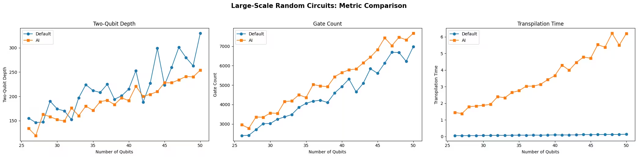
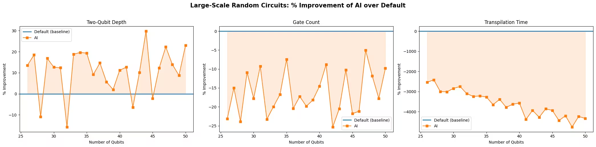
plot_metrics_and_pct(results_hw, "Large-Scale Random Circuits")

# -------------------------Step 3-------------------------
# Build mirror circuits from the 26-qubit case
idx_26q = qubit_range_hw.index(26)

qc_26q = circuits_hw[idx_26q]
qc_default_26q, _ = transpile_with_metrics(pm_default, qc_26q)

pm_ai = generate_ai_pass_manager(
    optimization_level=1,
    ai_optimization_level=3,
    backend=backend,
)
qc_ai_26q, _ = transpile_with_metrics(pm_ai, qc_26q)

mirror_default_hw = build_mirror_circuit(qc_default_26q, simulate=False)
mirror_ai_hw = build_mirror_circuit(qc_ai_26q, simulate=False)

# Re-transpile to basis gates (the inverse can introduce gates like sxdg)
pm_basis = generate_preset_pass_manager(
    optimization_level=0,
    backend=backend,
)
mirror_default_hw = pm_basis.run(mirror_default_hw)
mirror_ai_hw = pm_basis.run(mirror_ai_hw)

print(
    f"Mirror circuit (Default): depth {mirror_default_hw.depth()}, gates {mirror_default_hw.size()}"
)
print(
    f"Mirror circuit (AI):      depth {mirror_ai_hw.depth()}, gates {mirror_ai_hw.size()}"
)

# Submit to real hardware
sampler_hw = SamplerV2(mode=backend)
sampler_hw.options.environment.job_tags = ["TUT_AITI"]

shots_hw = 500000
job_hw = sampler_hw.run([mirror_default_hw, mirror_ai_hw], shots=shots_hw)
print(f"Job submitted: {job_hw.job_id()}")

Mirror circuit (Default): depth 1577, gates 9672
Mirror circuit (AI):      depth 1235, gates 11092
Job submitted: d8gt7vm6983c73dqbg0g

# -------------------------Step 4-------------------------
result_hw = job_hw.result()

survival_probs_hw = {}
for i, method in enumerate(["Default", "AI"]):
    counts = result_hw[i].data.meas.get_counts()
    mirror = [mirror_default_hw, mirror_ai_hw][i]
    all_zeros = "0" * mirror.num_qubits
    survival = counts.get(all_zeros, 0) / shots_hw
    survival_probs_hw[method] = survival
    print(
        f"{method:8s}  P(|00...0>) = {survival:.4f}  ({counts.get(all_zeros, 0)}/{shots_hw})"
    )

# Plot 1 - P(|0...0>), the probability of an erroneous (non-zero) outcome.
# A lower bar means the transpilation introduced less noise.
error_probs_hw = {method: 1 - p for method, p in survival_probs_hw.items()}

fig, ax = plt.subplots(figsize=(6, 4))
ax.bar(
    error_probs_hw.keys(),
    error_probs_hw.values(),
    color=["steelblue", "coral"],
)
ax.set_ylabel("1 - P(|0...0>)")
ax.set_title(f"Mirror Circuit Error (26-qubit, {backend.name})")
ax.set_ylim(0, 1)
plt.tight_layout()
plt.show()

Default   P(|00...0>) = 0.0005  (239/500000)
AI        P(|00...0>) = 0.0050  (2516/500000)

결과 분석

대규모 결과는 소규모 예제에서 관찰된 경향을 더욱 까다로운 규모에서 강화합니다.

두 Qubit 깊이: AI 기반 Transpiler는 Circuit 크기의 전 범위에 걸쳐 계속해서 눈에 띄게 낮은 두 Qubit 깊이를 제공합니다. 깊이 최적화는 AI 라우팅 모델이 훈련된 주요 목표 중 하나이며, 라우팅 문제가 휴리스틱 방법에 더 어려워지는 더 큰 Qubit 수에서 이점이 더 두드러집니다.

Gate 수: 기본 Transpiler(SABRE)는 이 범위의 모든 Circuit 크기에서 일관되게 더 적은 Gate를 가진 Circuit을 생성합니다. SABRE의 휴리스틱은 Gate 수를 최소화하도록 특별히 설계되어 있으며, 이 규모에서 그 이점이 명확하고 균일합니다.

트랜스파일 시간: 트랜스파일 시간의 격차는 더 큰 규모에서 벌어집니다. SABRE는 거의 일정하게 유지되는 반면, AI 기반 Transpiler의 런타임은 더 가파르게 증가합니다. 그럼에도 불구하고 AI 기반 Transpiler 런타임은 대부분의 워크플로우에서 실용적인 수준을 유지합니다.

미러 Circuit 충실도: 이 규모에서 두 방법 모두 생존 확률이 1% 미만으로, 사용 가능한 신호가 거의 없습니다. 총 Gate 수가 약 10,000개이고 두 Qubit 깊이가 1,000을 초과하면 미러 Circuit 전체에 걸쳐 누적된 탈분극 노이즈가 신호 대부분을 압도합니다. 이는 미러 Circuit 접근 방식의 주요 한계를 강조합니다: 단순하고 고전적 시뮬레이션이 필요 없지만, 두 방법 모두 노이즈 한계에 가까워지고 남아 있는 작은 신호가 누적된 오류에 의해 지배되는 대규모 또는 깊은 Circuit에는 잘 확장되지 않습니다.

이러한 결과는 AI 기반 Transpiler의 효과를 강조하지만, 그 한계를 주목하는 것이 중요합니다. AI 합성 방법은 현재 특정 커플링 맵에서만 사용 가능하여 더 넓은 적용 가능성을 제한할 수 있습니다. 이 제약은 다른 시나리오에서의 사용을 평가할 때 고려해야 합니다.

다음 단계

권장 사항

이 작업이 흥미로우셨다면 다음 자료에 관심이 있을 수 있습니다:

• SABRE를 사용한 트랜스파일 최적화
• 해밀토니안 시뮬레이션 Circuit을 위한 컴파일 방법