동적 회로를 이용한 장거리 얽힘
사용 시간 예상: Heron r2 프로세서 기준 약 4분. (참고: 이는 추정치이며, 실제 실행 시간은 다를 수 있습니다.)
학습 목표
이 튜토리얼을 완료하면 다음을 배우게 됩니다:
- 중간 회로 측정(MCM)과 고전적 피드포워드를 사용한 동적 회로로 장거리 CNOT Gate를 구현하는 방법;
- 유니터리 SWAP 기반 방식으로 동등한 Gate를 구현하는 방법;
- qubit 거리에 따른 Gate 충실도를 측정하여 두 방식을 비교하는 방법.
사전 지식
이 튜토리얼을 시작하기 전에 다음 주제에 익숙할 것을 권장합니다:
- Bell 상태, 얽힘, 양자 Gate를 포함한 기본 양자 컴퓨팅 개념;
- 동적 회로(중간 회로 측정 및 고전적 피드포워드)에 대한 이해;
- Qiskit SDK 및 Qiskit Runtime의 기본 지식과 IBM Quantum® 계정 접근 권한.
배경
먼 거리에 있는 큐비트들 사이의 장거리 얽힘은 연결성이 제한된 장치에서 구현하기 어렵습니다. 이 튜토리얼은 동적 회로가 측정 기반 프로토콜을 통해 장거리 제어-X (LRCX) 게이트를 구현함으로써 이러한 얽힘을 생성할 수 있는 방법을 보여줍니다.
Elisa Bäumer 등의 논문 1에서 제시된 방법을 따르며, 이 방법은 큐비트 간격에 관계없이 일정한 깊이의 게이트를 달성하기 위해 중간 회로 측정과 피드포워드를 활용합니다. 중간 Bell 쌍을 생성하고, 각 쌍에서 하나의 큐비트를 측정한 뒤, 클래식 조건부 게이트를 적용하여 장치 전체에 얽힘을 전파합니다. 이 방식은 긴 SWAP 체인을 피함으로써 회로 깊이와 2큐비트 게이트 오류 노출을 모두 줄입니다.
이 노트북에서는 IBM Quantum 하드웨어에 맞게 프로토콜을 적용하고, 제어-타겟 간격에 따른 성능을 벤치마킹하여 유니터리 SWAP 기반 기준선과 비교합니다.
요구 사항
이 튜토리얼을 시작하기 전에 다음 항목이 설치되어 있는지 확인하세요:
- Qiskit SDK v2.0 이상, 시각화 지원 포함
- Qiskit Runtime v0.37 이상 (
pip install qiskit-ibm-runtime) - Qiskit Aer v0.17 이상 (
pip install qiskit-aer)
설정
# Added by doQumentation — required packages for this notebook
!pip install -q matplotlib numpy qiskit qiskit-aer qiskit-ibm-runtime
from qiskit import QuantumCircuit, QuantumRegister, ClassicalRegister
from qiskit.circuit.classical import expr
from qiskit.transpiler import generate_preset_pass_manager
from qiskit.visualization import plot_circuit_layout
from qiskit_ibm_runtime import (
    QiskitRuntimeService,
    Batch,
    SamplerV2 as Sampler,
)
import matplotlib.pyplot as plt
import numpy as np
소규모 시뮬레이터 예제
실제 QPU에서 실행하기 전에, 노이즈가 없는 시뮬레이터에서 동적 회로와 유니터리 회로 모두 이상적인 Bell 상태를 생성하는지 확인합니다. 거리 6의 소규모 예제에서 AerSimulator를 Backend 모드로 사용하는 Qiskit Runtime Sampler를 사용합니다.
Step 1: 고전적 입력을 양자 문제로 변환하기
이제 두 멀리 떨어진 큐비트 사이에 장거리 CNOT 게이트를 구현합니다. 이는 아래에 나타난 동적 회로 구성 방식을 따릅니다 (참고문헌 1의 그림 1a에서 발췌). 핵심 아이디어는 으로 초기화된 보조 큐비트의 "버스"를 사용하여 장거리 게이트 텔레포테이션을 매개하는 것입니다.
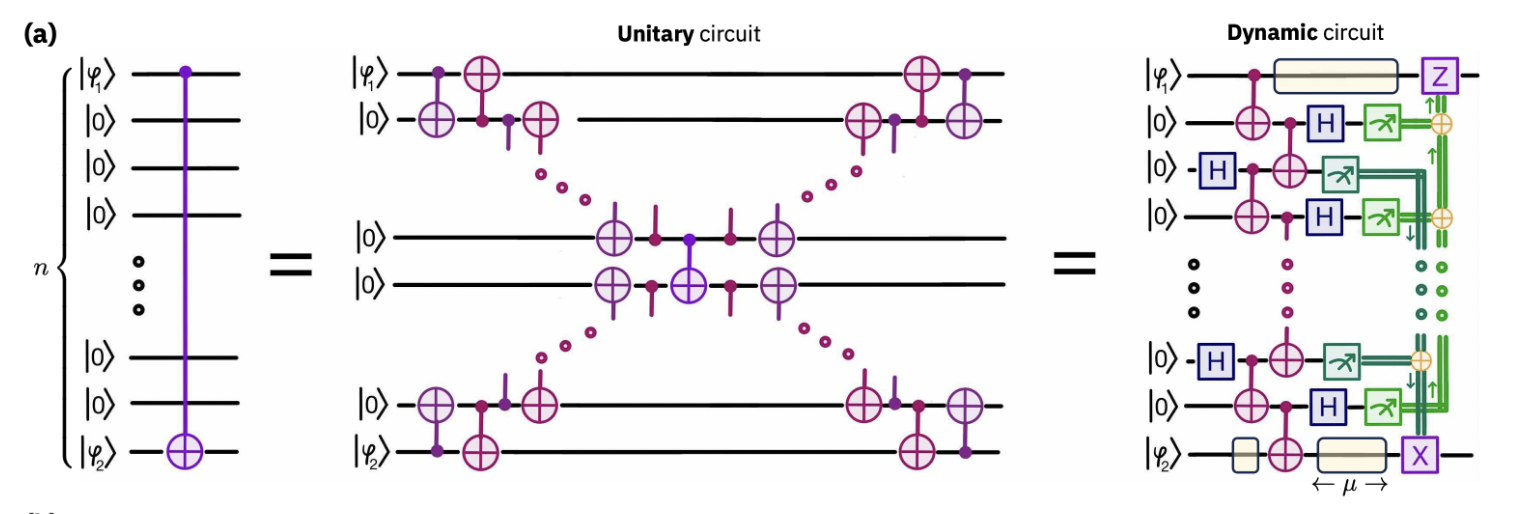
그림에서 보듯이, 이 과정은 다음과 같이 작동합니다:
- 중간 보조 큐비트를 통해 제어 큐비트와 타겟 큐비트를 연결하는 Bell 쌍 체인을 준비합니다.
- 얽히지 않은 인접 큐비트들 사이에서 Bell 측정을 수행하여, 제어 큐비트와 타겟 큐비트가 Bell 쌍을 공유할 때까지 단계적으로 얽힘을 교환합니다.
- 이 Bell 쌍을 사용하여 게이트 텔레포테이션을 수행하고, 지역적 CNOT을 일정 깊이에서 결정론적 장거리 CNOT으로 변환합니다.
이 접근법은 긴 SWAP 체인을 일정 깊이 프로토콜로 대체하여 2큐비트 게이트 오류 노출을 줄이고 장치 크기에 따라 확장 가능하게 만듭니다.
아래에서는 먼저 LRCX 회로의 동적 회로 구현을 단계별로 살펴봅니다. 마지막에는 비교를 위해 유니터리 기반 구현도 제공하여, 이 설정에서 동적 회로의 장점을 부각시킵니다.
회로 초기화
먼저 비교의 기준이 될 간단한 양자 문제로 시작합니다. 구체적으로, 인덱스 0의 제어 큐비트로 회로를 초기화하고 Hadamard 게이트를 적용합니다. 이를 통해 중첩 상태가 생성되며, 이후 제어-X 연산과 결합하면 제어 큐비트와 타겟 큐비트 사이에 Bell 상태 가 생성됩니다.
이 단계에서는 아직 장거리 제어-X (LRCX) 자체를 구성하지 않습니다. 대신, LRCX의 역할을 명확하게 보여주는 간단하고 최소한의 초기 회로를 정의하는 것이 목표입니다. Step 2에서는 LRCX를 동적 회로를 이용한 최적화로 구현하는 방법을 보여주고, 유니터리 등가물과 성능을 비교합니다. 중요한 점은 LRCX 프로토콜이 어떤 초기 회로에도 적용될 수 있다는 것입니다. 여기서는 설명의 명확성을 위해 이 간단한 Hadamard 설정을 사용합니다.
distance = 6  # The distance of the CNOT gate, with the convention that a distance of zero is a nearest-neighbor CNOT.

def initialize_circuit(distance):
    assert distance >= 0
    control = 0  # control qubit
    n = distance  # number of qubits between target and control

    qr = QuantumRegister(
        n + 2, name="q"
    )  # Circuit with n qubits between control and target
    cr = ClassicalRegister(
        2, name="cr"
    )  # Classical register for measuring control and target qubits

    k = int(n / 2)  # Number of Bell States to be used

    allcr = [cr]
    if (
        distance > 1
    ):  # This classical register will be used to store ZZ measurements.
        # It is only used for long-range CX gates with distance > 1
        c1 = ClassicalRegister(
            k, name="c1"
        )  # Classical register needed for post processing
        allcr.append(c1)
    if (
        distance > 0
    ):  # This classical register will be used to store XX measurements.
        # It is only used if distance > 0
        c2 = ClassicalRegister(
            n - k, name="c2"
        )  # Classical register needed for post processing
        allcr.append(c2)

    qc = QuantumCircuit(qr, *allcr, name="CNOT")

    # Apply a Hadamard gate to the control qubit such that the
    # long-range CNOT gate will prepare a
    # Bell state (|00> + |11>)/sqrt(2)
    qc.h(control)

    return qc

qc = initialize_circuit(distance)
qc.draw(fold=-1, output="mpl", scale=0.5)

Step 2: 양자 하드웨어 실행을 위한 문제 최적화
이 단계에서는 동적 회로(dynamic circuits)를 사용하여 LRCX 회로를 구성하는 방법을 보여줍니다. 목표는 순수 유니타리 구현에 비해 깊이(depth)를 줄임으로써 하드웨어 실행에 맞게 회로를 최적화하는 것입니다. 이점을 명확히 보여주기 위해 동적 LRCX 구성과 그에 상응하는 유니타리 버전을 모두 표시하고, 나중에 트랜스파일 후 성능을 비교합니다. 중요한 점은, 여기서는 LRCX를 간단한 Hadamard 초기화 문제에 적용하지만, 이 프로토콜은 장거리 CNOT이 필요한 모든 회로에 적용할 수 있다는 것입니다.
Bell 쌍 준비
먼저 제어 Qubit과 타겟 qubit 사이의 경로를 따라 Bell 쌍 체인을 생성합니다. 거리가 홀수인 경우, 먼저 제어 Qubit에서 인접 Qubit으로 CNOT을 적용하는데, 이것이 텔레포트될 CNOT입니다. 거리가 짝수인 경우, 이 CNOT은 Bell 쌍 준비 단계 이후에 적용됩니다. 그런 다음 Bell 쌍 체인이 연속된 qubit 쌍을 얽히게 하여, 제어 정보를 장치 전체에 전달하는 데 필요한 리소스를 구축합니다.
# Determine where to start the Bell pair chain and add an extra CNOT when n is odd
def check_even(n: int) -> int:
    """Return 1 if n is even, else 2."""
    return 1 if n % 2 == 0 else 2

def prepare_bell_pairs(qc, add_barriers=True):
    n = qc.num_qubits - 2  # number of qubits between target and control
    k = int(n / 2)

    if add_barriers:
        qc.barrier()

    x0 = check_even(n)
    if n % 2 != 0:
        qc.cx(0, 1)

    # Create k Bell pairs
    for i in range(k):
        qc.h(x0 + 2 * i)
        qc.cx(x0 + 2 * i, x0 + 2 * i + 1)
    return qc

qc = prepare_bell_pairs(qc)
qc.draw(output="mpl", fold=-1, scale=0.5)

Bell 기저에서 인접 qubit 쌍 측정
다음으로, 얽히지 않은 인접 Qubit들을 Bell 기저( 및 의 두 qubit 측정)에서 측정합니다. 이를 통해 타겟 Qubit과 제어 Qubit에 인접한 qubit 사이에 장거리 Bell 쌍이 생성됩니다(Pauli 보정은 다음 단계에서 피드포워드를 통해 구현됩니다). 이와 동시에, CNOT Gate를 의도한 타겟 Qubit에 작용하도록 텔레포트하는 얽힘 측정을 구현합니다.
def measure_bell_basis(qc, add_barriers=True):
    n = qc.num_qubits - 2  # number of qubits between target and control
    k = int(n / 2)

    if n > 1:
        _, c1, c2 = qc.cregs
    elif n > 0:
        _, c2 = qc.cregs

    # Determine where to start the Bell pair chain and add an extra CNOT
    # when n is odd
    x0 = 1 if n % 2 == 0 else 2

    # Entangling layer that implements the Bell measurement
    # (and additionally adds the CNOT to be
    # teleported, if n is even)
    for i in range(k + 1):
        qc.cx(x0 - 1 + 2 * i, x0 + 2 * i)

    for i in range(1, k + x0):
        if i == 1:
            qc.h(2 * i + 1 - x0)
        else:
            qc.h(2 * i + 1 - x0)

    if add_barriers:
        qc.barrier()

    # Map the ZZ measurements onto classical register c1
    for i in range(k):
        if i == 0:
            qc.measure(2 * i + x0, c1[i])
        else:
            qc.measure(2 * i + x0, c1[i])

    # Map the XX measurements onto classical register c2
    for i in range(1, k + x0):
        if i == 1:
            qc.measure(2 * i + 1 - x0, c2[i - 1])
        else:
            qc.measure(2 * i + 1 - x0, c2[i - 1])
    return qc

qc = measure_bell_basis(qc)
qc.draw(output="mpl", fold=-1, scale=0.5)

Pauli 부산물 연산자 보정을 위한 피드포워드 적용
Bell 기저 측정은 기록된 결과를 사용하여 보정해야 하는 Pauli 부산물을 도입합니다. 이는 두 단계로 수행됩니다. 먼저 모든 측정의 패리티를 계산해야 하며, 이를 사용하여 타겟 Qubit에 Gate를 조건부로 적용합니다. 마찬가지로, 측정의 패리티를 계산하여 제어 Qubit에 Gate를 조건부로 적용합니다.
Qiskit의 새로운 고전 표현식 프레임워크를 사용하면 이러한 패리티를 회로의 고전 처리 레이어에서 직접 계산할 수 있습니다. 각 측정 비트에 대해 개별 조건부 Gate 시퀀스를 적용하는 대신, 모든 관련 측정 결과의 XOR(패리티)를 나타내는 단일 고전 표현식을 구성할 수 있습니다. 이 표현식은 단일 if_test 블록의 조건으로 사용되어, 보정 Gate를 상수 깊이로 적용할 수 있습니다. 이 방식은 회로를 단순화하고 피드포워드 보정이 불필요한 추가 지연을 도입하지 않도록 보장합니다.
def apply_ffwd_corrections(qc):
    control = 0  # control qubit
    target = qc.num_qubits - 1  # target qubit
    n = qc.num_qubits - 2  # number of qubits between target and control

    k = int(n / 2)
    x0 = check_even(n)

    if n > 1:
        _, c1, c2 = qc.cregs
    elif n > 0:
        _, c2 = qc.cregs

    # First, let's compute the parity of all ZZ measurements
    for i in range(k):
        if i == 0:
            parity_ZZ = expr.lift(
                c1[i]
            )  # Store the value of the first ZZ measurement in parity_ZZ
        else:
            parity_ZZ = expr.bit_xor(
                c1[i], parity_ZZ
            )  # Successively compute the parity via XOR operations

    for i in range(1, k + x0):
        if i == 1:
            parity_XX = expr.lift(
                c2[i - 1]
            )  # Store the value of the first XX measurement in parity_XX
        else:
            parity_XX = expr.bit_xor(
                c2[i - 1], parity_XX
            )  # Successively compute the parity via XOR operations

    if n > 0:
        with qc.if_test(parity_XX):
            qc.z(control)

    if n > 1:
        with qc.if_test(parity_ZZ):
            qc.x(target)
    return qc

qc = apply_ffwd_corrections(qc)
qc.draw(output="mpl", fold=-1, scale=0.5)

제어 및 타겟 qubit 측정
, , 또는 기저에서 제어 및 타겟 Qubit의 측정을 가능하게 하는 헬퍼 함수를 정의합니다. Bell 상태 를 검증하기 위해 와 의 기댓값은 모두 이어야 하는데, 이들이 해당 상태의 안정자(stabilizer)이기 때문입니다. 측정도 여기서 지원되며, 아래에서 충실도(fidelity)를 계산할 때 사용됩니다.
def measure_in_basis(qc, basis="XX", add_barrier=True):
    control = 0  # control qubit
    target = qc.num_qubits - 1  # target qubit

    assert basis in ["XX", "YY", "ZZ"]

    qc = (
        qc.copy()
    )  # We copy the circuit because we want to measure in different bases
    cr = qc.cregs[0]

    if add_barrier:
        qc.barrier()

    if basis == "XX":
        qc.h(control)
        qc.h(target)
    elif basis == "YY":
        qc.sdg(control)
        qc.sdg(target)
        qc.h(control)
        qc.h(target)

    qc.measure(control, cr[0])
    qc.measure(target, cr[1])
    return qc

qc_YY = measure_in_basis(qc.copy(), basis="YY")
qc_YY.draw(
    output="mpl", fold=-1, scale=0.5
)  # Circuit for measuring in the YY basis

모든 단계 합치기
위에서 정의한 다양한 단계들을 결합하여 1차원(1D) 라인의 양 끝에 있는 두 qubit 사이에 장거리 CX Gate를 생성합니다. 단계는 다음과 같습니다:
- 제어 Qubit을 상태로 초기화
- Bell 쌍 준비
- 이웃 qubit 쌍 측정
- MCM에 의존하는 피드포워드 보정 적용
def lrcx(distance, prep_barrier=True, pre_measure_barrier=True):
    qc = initialize_circuit(distance)
    qc = prepare_bell_pairs(qc, prep_barrier)
    qc = measure_bell_basis(qc, pre_measure_barrier)
    qc = apply_ffwd_corrections(qc)
    return qc

qc = lrcx(distance)
# Apply the measurement in the XX, YY, and ZZ bases
qc_XX, qc_YY, qc_ZZ = [
    measure_in_basis(qc, basis=basis) for basis in ["XX", "YY", "ZZ"]
]

qc_YY.draw(
    output="mpl", fold=-1, scale=0.5
)  # Circuit for measuring in the YY basis
Qubit을 중앙으로 스왑하는 유니터리 기반 구현
비교를 위해, 먼저 최근접 이웃 연결과 유니터리 Gate를 사용하여 장거리 CNOT Gate를 구현하는 경우를 살펴봅니다. 아래 그림에서 왼쪽은 최근접 이웃 연결만 허용되는 n-Qubit 1D 체인에 걸쳐 있는 장거리 CNOT Gate의 Circuit이고, 가운데는 로컬 CNOT Gate로 구현 가능한 동등한 유니터리 분해로, Circuit 깊이는 입니다.
가운데 Circuit은 다음과 같이 구현할 수 있습니다:
def cnot_unitary(distance):
    """Generate a long range CNOT gate using local CNOTs on a 1D
    chain of qubits subject to n
    nearest-neighbor connections only.

    Args:
        distance (int) : The distance of the CNOT gate,
        with the convention that
        a distance of 0 is a nearest-neighbor CNOT.

    Returns:
        QuantumCircuit: A Quantum Circuit implementing a
        long-range CNOT gate
        between qubit 0 and qubit distance+1
    """
    assert distance >= 0
    n = distance  # number of qubits between target and control

    qr = QuantumRegister(
        n + 2, name="q"
    )  # Circuit with n qubits between control and target
    cr = ClassicalRegister(
        2, name="cr"
    )  # Classical register for measuring control and target qubits

    qc = QuantumCircuit(qr, cr, name="CNOT_unitary")

    control_qubit = 0

    qc.h(control_qubit)  # Prepare the control qubit in the |+> state

    k = int(n / 2)
    qc.barrier()
    for i in range(control_qubit, control_qubit + k):
        qc.cx(i, i + 1)
        qc.cx(i + 1, i)
        qc.cx(-i - 1, -i - 2)
        qc.cx(-i - 2, -i - 1)
    if n % 2 == 1:
        qc.cx(k + 2, k + 1)
        qc.cx(k + 1, k + 2)
    qc.barrier()
    qc.cx(k, k + 1)
    for i in range(control_qubit, control_qubit + k):
        qc.cx(k - i, k - 1 - i)
        qc.cx(k - 1 - i, k - i)
        qc.cx(k + i + 1, k + i + 2)
        qc.cx(k + i + 2, k + i + 1)
    if n % 2 == 1:
        qc.cx(-2, -1)
        qc.cx(-1, -2)

    return qc

qc_uni = cnot_unitary(distance)
이제 위에서 동적 Circuit에 대해 했던 것처럼 , , 기저에서 측정하는 Circuit을 구성합니다.
# Apply the measurement in the XX, YY, and ZZ bases
qc_uni_XX, qc_uni_YY, qc_uni_ZZ = [
    measure_in_basis(qc_uni, basis=basis) for basis in ["XX", "YY", "ZZ"]
]

qc_uni_YY.draw(
    output="mpl", fold=-1, scale=0.5
)  # Circuit for measuring in the YY basis

이제 distance=6의 소규모 예제에서 동적 Circuit과 유니터리 Circuit을 모두 구성했으므로, 먼저 노이즈 없는 시뮬레이터에서 실행하기 위해 트랜스파일합니다.
from qiskit_aer import AerSimulator

aer_backend = AerSimulator()
pm_sim = generate_preset_pass_manager(
    optimization_level=0, backend=aer_backend
)

# Dynamic circuits
isa_sim_dyn = pm_sim.run([qc_XX, qc_YY, qc_ZZ])

# Unitary circuits
isa_sim_uni = pm_sim.run([qc_uni_XX, qc_uni_YY, qc_uni_ZZ])
Step 3: Qiskit 프리미티브를 사용한 실행
이제 노이즈 없는 시뮬레이터 Backend에서 실험을 실행할 수 있습니다. AerSimulator를 Backend 모드로 사용하는 Qiskit Runtime Sampler를 활용해 Circuit을 실행합니다.
sampler_sim = Sampler(mode=aer_backend)
sim_job = sampler_sim.run(isa_sim_dyn + isa_sim_uni)
sim_results = sim_job.result()
Step 4: 후처리 및 원하는 고전적 형식으로 결과 반환
실험이 성공적으로 실행된 후, 이제 측정 카운트를 후처리하여 의미 있는 지표를 추출합니다. 이 단계에서는 다음을 수행합니다:
- 장거리 CX의 성능을 평가하기 위한 품질 지표를 정의합니다.
- 원시 측정 결과에서 Pauli 연산자의 기댓값을 계산합니다.
- 이를 사용하여 생성된 Bell 상태의 충실도(fidelity)를 계산합니다.
노이즈 없는 시뮬레이션에서는 구성된 Circuit의 충실도 지표가 임을 확인할 것입니다. 실제 QPU에서의 실험에서 이 분석은 동적 Circuit이 유니터리 기준 구현과 비교하여 얼마나 잘 수행되는지를 명확하게 보여줄 것입니다.
품질 지표
장거리 CX 프로토콜의 성공 여부를 평가하기 위해, 출력 상태가 이상적인 Bell 상태에 얼마나 가까운지를 측정합니다. 이를 정량화하는 편리한 방법은 Pauli 연산자의 기댓값을 사용하여 상태 충실도를 계산하는 것입니다. 제어 및 타겟 상태에 대한 Bell 상태의 충실도는 , , 를 알면 계산할 수 있습니다. 구체적으로,
원시 측정 데이터에서 이러한 기댓값을 계산하기 위해 다음과 같은 보조 함수들을 정의합니다:
compute_ZZ_expectation: 측정 카운트가 주어지면 기저에서 2-Qubit Pauli 연산자의 기댓값을 계산합니다.compute_fidelity: , , 의 기댓값을 위의 충실도 표현식으로 결합합니다.get_counts_from_bitarray: Backend 결과 객체에서 카운트를 추출하는 유틸리티입니다.
def compute_ZZ_expectation(counts):
    total = sum(counts.values())
    expectation = 0
    for bitstring, count in counts.items():
        # Ensure bitstring is 2 bits
        z1 = (-1) ** (int(bitstring[-1]))
        z2 = (-1) ** (int(bitstring[-2]))
        expectation += z1 * z2 * count
    return expectation / total

def compute_fidelity(counts_xx, counts_yy, counts_zz):
    xx, yy, zz = [
        compute_ZZ_expectation(c) for c in [counts_xx, counts_yy, counts_zz]
    ]
    return 1 / 4 * (1 + xx - yy + zz)
# Dynamic fidelity
counts_xx = sim_results[0].data.cr.get_counts()
counts_yy = sim_results[1].data.cr.get_counts()
counts_zz = sim_results[2].data.cr.get_counts()
fidelity_dyn = compute_fidelity(counts_xx, counts_yy, counts_zz)

# Unitary fidelity
counts_xx = sim_results[3].data.cr.get_counts()
counts_yy = sim_results[4].data.cr.get_counts()
counts_zz = sim_results[5].data.cr.get_counts()
fidelity_uni = compute_fidelity(counts_xx, counts_yy, counts_zz)

print(f"Dynamic fidelity (distance={distance}): {fidelity_dyn:.4f}")
print(f"Unitary fidelity (distance={distance}): {fidelity_uni:.4f}")
Dynamic fidelity (distance=6): 1.0000
Unitary fidelity (distance=6): 1.0000
노이즈 없는 시뮬레이션에서 예상대로, 동적 Circuit과 유니터리 Circuit 모두 충실도가 입니다.
대규모 하드웨어 예제
이제 이 모든 세부 사항을 더 큰 규모의 단일 워크플로우로 통합하여 실제 양자 하드웨어에서 실행합니다.
다양한 거리에 대한 Circuit 생성
이제 최대 60 qubit 간격에 걸쳐 다양한 qubit 간격에 대해 장거리 CX Circuit을 생성합니다. 각 거리에 대해 , , 기저에서 측정하는 Circuit을 구성하며, 이는 나중에 충실도(fidelity)를 계산하는 데 사용됩니다.
거리 목록에는 단거리와 장거리 간격이 모두 포함되어 있으며, distance = 0은 최근접 이웃 CX에 해당합니다. 이 동일한 거리들은 나중에 비교를 위해 해당하는 유니터리 Circuit을 생성하는 데도 사용됩니다.
# -------------------------Step 1-------------------------
distances = [
    0,
    1,
    2,
    3,
    6,
    11,
    16,
    21,
    28,
    35,
    44,
    55,
    60,
]  # Distances for long range CX. distance of 0 is a nearest-neighbor CX
distances.sort()
assert min(distances) >= 0
basis_list = ["XX", "YY", "ZZ"]

# Dynamic circuits
circuits_dyn = []
for distance in distances:
    for basis in basis_list:
        circuits_dyn.append(
            measure_in_basis(lrcx(distance, prep_barrier=False), basis=basis)
        )
print(f"Number of circuits: {len(circuits_dyn)}")

# Unitary circuits
circuits_uni = []
for distance in distances:
    for basis in basis_list:
        circuits_uni.append(
            measure_in_basis(cnot_unitary(distance), basis=basis)
        )

print(f"Number of circuits: {len(circuits_uni)}")
# -------------------------Step 2-------------------------
# Set up access to IBM Quantum devices
from qiskit.circuit import IfElseOp

service = QiskitRuntimeService()
backend = service.least_busy(
    operational=True, simulator=False, min_num_qubits=156
)
if "if_else" not in backend.target.operation_names:
    backend.target.add_instruction(IfElseOp, name="if_else")
1D 체인 선택을 위한 Layer Fidelity 문자열 사용
동적 회로와 unitary 회로의 성능을 1D 체인에서 비교하고자 하므로, Layer Fidelity 문자열을 사용하여 디바이스에서 가장 좋은 qubit 체인의 선형 토폴로지를 선택합니다. 이렇게 하면 두 유형의 회로가 동일한 연결성 제약 조건 하에서 트랜스파일되어 성능을 공정하게 비교할 수 있습니다.
# This selects best qubits for longest distance and uses
# the same control for all lengths
lf_qubits = backend.properties().to_dict()[
    "general_qlists"
]  # best linear chain qubits
chosen_layouts = {
    distance: [
        val["qubits"]
        for val in lf_qubits
        if val["name"] == f"lf_{distances[-1] + 2}"
    ][0][: distance + 2]
    for distance in distances
}
print(chosen_layouts[max(distances)])  # best qubits at each distance
[11, 12, 13, 14, 15, 19, 35, 34, 33, 39, 53, 54, 55, 59, 75, 74, 73, 72, 71, 70, 69, 68, 67, 66, 65, 64, 63, 62, 61, 76, 81, 82, 83, 84, 85, 86, 87, 97, 107, 108, 109, 110, 111, 98, 91, 92, 93, 94, 95, 99, 115, 114, 113, 119, 133, 132, 131, 138, 151, 150, 149, 148]
isa_circuits_dyn = []
isa_circuits_uni = []

# Using the same initial layouts for both circuits for better
# apples to apples comparison
for qc in circuits_dyn:
    pm = generate_preset_pass_manager(
        optimization_level=1,
        backend=backend,
        initial_layout=chosen_layouts[qc.num_qubits - 2],
    )
    isa_circuits_dyn.append(pm.run(qc))

for qc in circuits_uni:
    pm = generate_preset_pass_manager(
        optimization_level=1,
        backend=backend,
        initial_layout=chosen_layouts[qc.num_qubits - 2],
    )
    isa_circuits_uni.append(pm.run(qc))
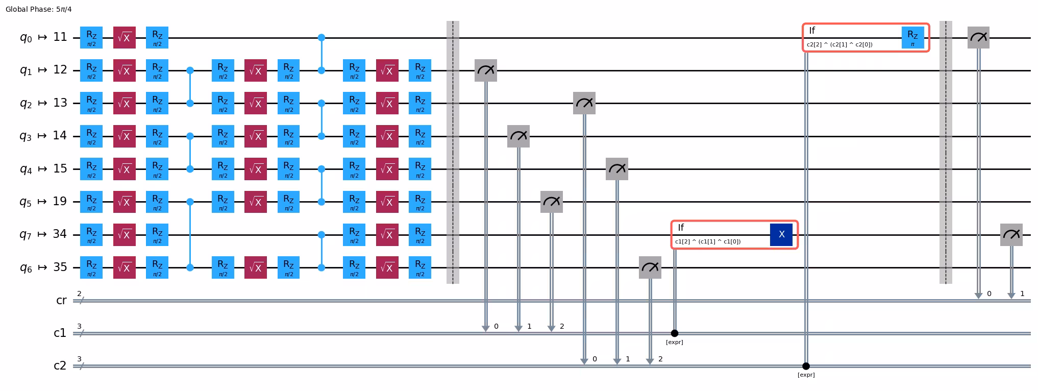
print(
    f"2Q depth: "
    f"{isa_circuits_dyn[14].depth(lambda x: x.operation.num_qubits == 2)}"
)
isa_circuits_dyn[14].draw("mpl", fold=-1, idle_wires=0)
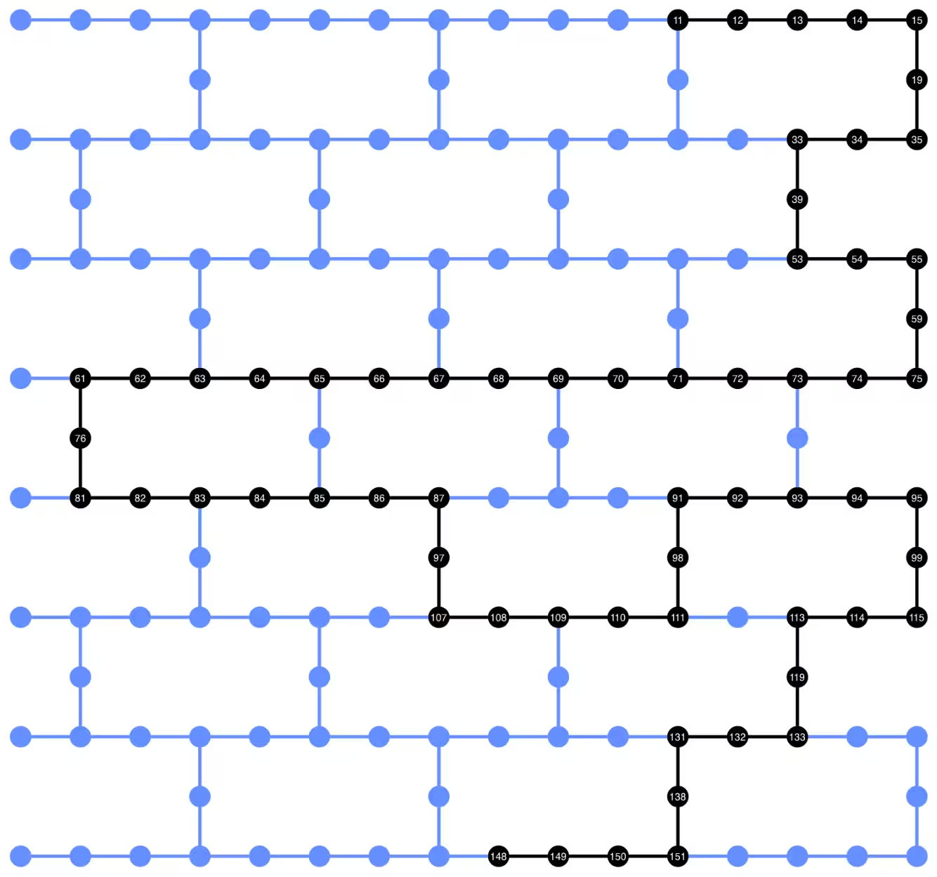
LRCX Circuit에 사용된 qubit 시각화
이 섹션에서는 LRCX Circuit이 하드웨어에 어떻게 매핑되는지 살펴봅니다. 먼저 Circuit에 사용된 물리적 Qubit을 시각화한 다음, 레이아웃에서 제어-타겟 간 거리가 연산 횟수에 미치는 영향을 분석합니다.
2Q depth: 2
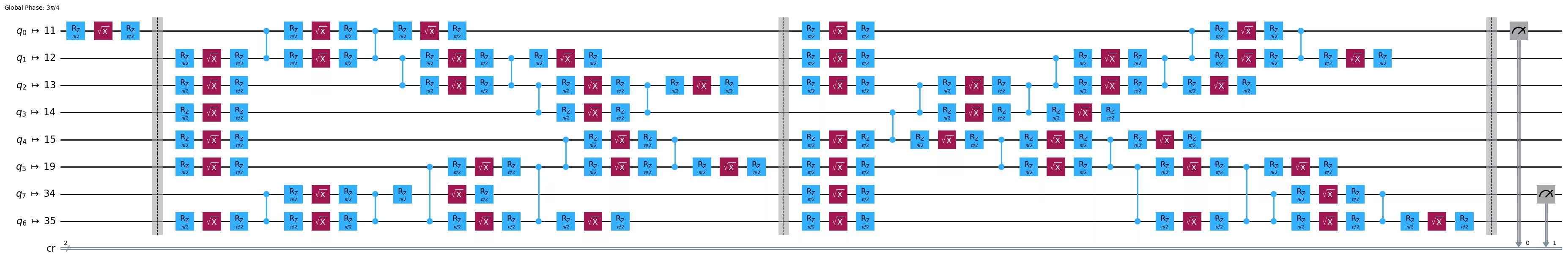
print(
    f"2Q depth: "
    f"{isa_circuits_uni[14].depth(lambda x: x.operation.num_qubits == 2)}"
)
isa_circuits_uni[14].draw("mpl", fold=-1, idle_wires=False)
2Q depth: 13
다음으로, 실제 Backend에서 실험을 실행합니다. 또한 배치(batching)를 활용하여 여러 시행(trial)에 걸쳐 실험을 효율적으로 수행합니다. 반복 시행을 통해 단일(unitary) 방법과 동적(dynamic) 방법 간의 평균값을 계산하여 더 정확한 비교를 할 수 있으며, 시행 간 편차를 비교해 변동성을 정량화할 수 있습니다.
# Note: the qubit coordinates must be hard-coded.
# The backend API does not currently provide this information directly.
# If using a different backend, you will need to
# adjust the coordinates accordingly,
# or set the qubit_coordinates = None to use the default layout coordinates.

def _heron_coords_r2():
    """Generate coordinates for the Heron layout in R2. Note"""
    cord_map = np.array(
        [
            [
                0,
                1,
                2,
                3,
                4,
                5,
                6,
                7,
                8,
                9,
                10,
                11,
                12,
                13,
                14,
                15,
                3,
                7,
                11,
                15,
                0,
                1,
                2,
                3,
                4,
                5,
                6,
                7,
                8,
                9,
                10,
                11,
                12,
                13,
                14,
                15,
                1,
                5,
                9,
                13,
                0,
                1,
                2,
                3,
                4,
                5,
                6,
                7,
                8,
                9,
                10,
                11,
                12,
                13,
                14,
                15,
                3,
                7,
                11,
                15,
                0,
                1,
                2,
                3,
                4,
                5,
                6,
                7,
                8,
                9,
                10,
                11,
                12,
                13,
                14,
                15,
                1,
                5,
                9,
                13,
                0,
                1,
                2,
                3,
                4,
                5,
                6,
                7,
                8,
                9,
                10,
                11,
                12,
                13,
                14,
                15,
                3,
                7,
                11,
                15,
                0,
                1,
                2,
                3,
                4,
                5,
                6,
                7,
                8,
                9,
                10,
                11,
                12,
                13,
                14,
                15,
                1,
                5,
                9,
                13,
                0,
                1,
                2,
                3,
                4,
                5,
                6,
                7,
                8,
                9,
                10,
                11,
                12,
                13,
                14,
                15,
                3,
                7,
                11,
                15,
                0,
                1,
                2,
                3,
                4,
                5,
                6,
                7,
                8,
                9,
                10,
                11,
                12,
                13,
                14,
                15,
            ],
            -1
            * np.array([j for i in range(15) for j in [i] * [16, 4][i % 2]]),
        ],
        dtype=int,
    )

    hcords = []
    ycords = cord_map[0]
    xcords = cord_map[1]
    for i in range(156):
        hcords.append([xcords[i] + 1, np.abs(ycords[i]) + 1])

    return hcords

# Visualize the active qubits in the circuit layout
plot_circuit_layout(
    circuit=isa_circuits_uni[-1],
    backend=backend,
    view="physical",
    qubit_coordinates=_heron_coords_r2(),
)
# -------------------------Step 3-------------------------
num_trials = 10
jobs_uni = []
jobs_dyn = []
with Batch(backend=backend) as batch:
    sampler = Sampler(mode=batch)
    sampler.options.environment.job_tags = ["TUT_LRE"]
    for _ in range(num_trials):
        jobs_uni.append(sampler.run(isa_circuits_uni, shots=1024))
        jobs_dyn.append(sampler.run(isa_circuits_dyn, shots=1024))
동적 장거리 CX Circuit의 충실도를 계산합니다. 각 거리에 대해 , , 기저의 측정 결과를 추출합니다. 이 결과는 앞서 정의한 보조 함수를 사용하여 에 따라 충실도를 계산하는 데 결합됩니다. 이를 통해 각 거리에서 동적 프로토콜의 관측 충실도를 얻을 수 있습니다.
# -------------------------Step 4-------------------------
fidelities_dyn = []

# loop over trials
for job in jobs_dyn:
    result_dyn = job.result()
    trial_fidelities = []
    # loop over all distances
    for ind, dist in enumerate(distances):
        counts_xx = result_dyn[ind * 3].data.cr.get_counts()
        counts_yy = result_dyn[ind * 3 + 1].data.cr.get_counts()
        counts_zz = result_dyn[ind * 3 + 2].data.cr.get_counts()
        trial_fidelities.append(
            compute_fidelity(counts_xx, counts_yy, counts_zz)
        )
    fidelities_dyn.append(trial_fidelities)
# average over trials for each distance
avg_fidelities_dyn = np.mean(fidelities_dyn, axis=0)
std_fidelities_dyn = np.std(fidelities_dyn, axis=0)
이제 단일(unitary) 장거리 CX Circuit의 충실도를 계산합니다. 동적 Circuit과 동일한 방식으로 수행합니다.
fidelities_uni = []

# loop over trials
for job in jobs_uni:
    result_uni = job.result()
    trial_fidelities = []
    # loop over all distances
    for ind, dist in enumerate(distances):
        counts_xx = result_uni[ind * 3].data.cr.get_counts()
        counts_yy = result_uni[ind * 3 + 1].data.cr.get_counts()
        counts_zz = result_uni[ind * 3 + 2].data.cr.get_counts()
        trial_fidelities.append(
            compute_fidelity(counts_xx, counts_yy, counts_zz)
        )
    fidelities_uni.append(trial_fidelities)
# average over trials for each distance
avg_fidelities_uni = np.mean(fidelities_uni, axis=0)
std_fidelities_uni = np.std(fidelities_uni, axis=0)
결과 시각화
아래 셀은 각 방법에 대해 얽힌 qubit 간의 거리에 따라 측정된 Gate 충실도 추정치를 시각적으로 보여줍니다.
fig, ax = plt.subplots()

# Unitary with error bars
ax.errorbar(
    distances,
    avg_fidelities_uni,
    yerr=std_fidelities_uni,
    fmt="o-.",
    color="c",
    ecolor="c",
    elinewidth=1,
    capsize=4,
    label="Unitary",
)
# Dynamic with error bars
ax.errorbar(
    distances,
    avg_fidelities_dyn,
    yerr=std_fidelities_dyn,
    fmt="o-.",
    color="m",
    ecolor="m",
    elinewidth=1,
    capsize=4,
    label="Dynamic",
)
# Random gate baseline
ax.axhline(y=1 / 4, linestyle="--", color="gray", label="Random gate")

legend = ax.legend(frameon=True)
for text in legend.get_texts():
    text.set_color("black")
legend.get_frame().set_facecolor("white")
legend.get_frame().set_edgecolor("black")
ax.set_title(
    "Bell State Fidelity vs Control–Target Separation", color="black"
)
ax.set_xlabel("Distance", color="black")
ax.set_ylabel("Bell state fidelity", color="black")
ax.grid(linestyle=":", linewidth=0.6, alpha=0.4, color="gray")
ax.set_ylim((0.2, 1))
ax.set_facecolor("white")
fig.patch.set_facecolor("white")
for spine in ax.spines.values():
    spine.set_visible(True)
    spine.set_color("black")
ax.tick_params(axis="x", colors="black")
ax.tick_params(axis="y", colors="black")
plt.show()
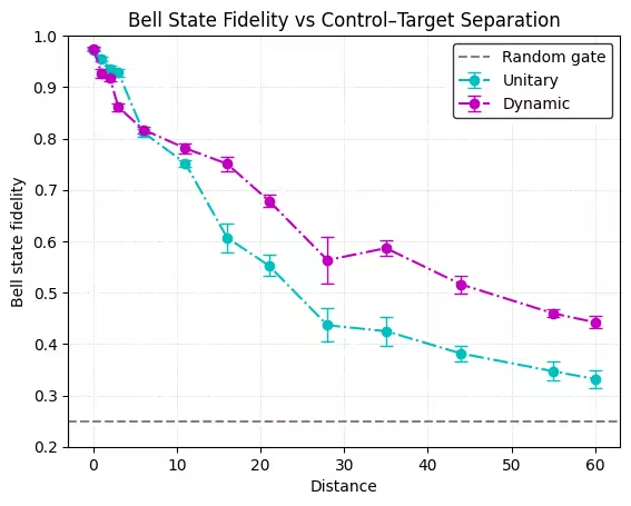
위의 충실도 그래프에서 LRCX는 직접 단일(unitary) 구현보다 일관되게 우수한 성능을 보이지 않았습니다. 실제로 제어-타겟 간 거리가 짧을 때는 단일 Circuit이 더 높은 충실도를 달성했습니다. 그러나 거리가 커질수록 동적 Circuit이 단일 구현보다 나은 충실도를 보이기 시작합니다. 이러한 동작은 현재 하드웨어에서 예상치 못한 것이 아닙니다. 동적 Circuit은 긴 SWAP 체인을 피함으로써 Circuit 깊이를 줄이지만, 중간 Circuit 측정, 고전적 피드포워드, 제어 경로 지연으로 인해 추가적인 Circuit 시간이 발생합니다. 이러한 추가 지연은 디코히런스와 판독 오류를 증가시켜 짧은 거리에서는 깊이 절약 효과보다 더 큰 영향을 미칠 수 있습니다.
그럼에도 불구하고, 동적 방법이 단일 방법을 능가하는 교차점을 관찰할 수 있습니다. 이는 서로 다른 스케일링의 직접적인 결과입니다. 단일 Circuit의 깊이는 qubit 간 거리에 따라 선형적으로 증가하는 반면, 동적 Circuit의 깊이는 일정하게 유지됩니다.
핵심 사항:
- 동적 Circuit의 즉각적인 이점: 오늘날 주요 동기는 충실도 향상이 아닌 2-Qubit 깊이 감소입니다.
- 오늘날 충실도가 낮을 수 있는 이유: 측정 및 고전적 연산으로 인한 Circuit 시간 증가가 지배적이며, 특히 제어-타겟 간 거리가 짧을 때 두드러집니다.
- 앞으로의 전망: 하드웨어가 개선됨에 따라, 특히 더 빠른 판독, 더 짧은 고전적 제어 지연, 중간 Circuit 오버헤드 감소가 이루어지면, 이러한 깊이 및 실행 시간 감소가 측정 가능한 충실도 향상으로 이어질 것으로 기대됩니다.
# Compute metrics for each distance, skipping the basis circuits since
# they are identical for each distance
depths_2q_dyn = [
    c.depth(lambda x: x.operation.num_qubits == 2)
    for c in isa_circuits_dyn[::3]
]
meas_dyn = [
    sum(1 for instr in c.data if instr.operation.name == "measure")
    for c in isa_circuits_dyn[::3]
]

depths_2q_uni = [
    c.depth(lambda x: x.operation.num_qubits == 2)
    for c in isa_circuits_uni[::3]
]
meas_uni = [
    sum(1 for instr in c.data if instr.operation.name == "measure")
    for c in isa_circuits_uni[::3]
]

fig, axes = plt.subplots(1, 2, figsize=(12, 5))

axes[0].plot(
    distances, depths_2q_uni, "o-.", color="c", label="Unitary (2Q depth)"
)
axes[0].plot(
    distances, depths_2q_dyn, "o-.", color="m", label="Dynamic (2Q depth)"
)
axes[0].set_xlabel("Number of qubits between control and target")
axes[0].set_ylabel("Two-qubit depth")
axes[0].grid(True, linestyle=":", linewidth=0.6, alpha=0.4)
axes[0].legend()

axes[1].plot(
    distances, meas_uni, "o-.", color="c", label="Unitary (# measurements)"
)
axes[1].plot(
    distances, meas_dyn, "o-.", color="m", label="Dynamic (# measurements)"
)
axes[1].set_xlabel("Number of qubits between control and target")
axes[1].set_ylabel("Number of measurements")
axes[1].grid(True, linestyle=":", linewidth=0.6, alpha=0.4)
axes[1].legend()

fig.suptitle("Scaling of Unitary vs Dynamic LRCX with Distance", fontsize=12)

plt.tight_layout()
plt.show()
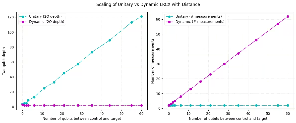
이 2-Qubit 깊이 그래프는 동적 Circuit으로 구현된 LRCX의 주요 장점을 강조합니다. 제어와 타겟 qubit 간의 거리가 증가해도 성능이 본질적으로 일정하게 유지됩니다. 반면, 단일 구현은 필요한 SWAP 체인으로 인해 거리에 따라 선형적으로 증가합니다. 깊이는 2-Qubit 연산의 논리적 스케일링을 나타내며, 측정 횟수는 동적 Circuit의 추가 오버헤드를 반영합니다. 이러한 측정은 병렬로 수행되어 효율적이지만, 오늘날 하드웨어에서는 고정 비용을 발생시킵니다.
오늘날 충실도가 낮을 수 있는 이유: 측정 및 고전적 연산으로 인한 Circuit 시간 증가가 지배적이며, 특히 제어-타겟 간 거리가 짧을 때 두드러집니다. 예를 들어, Heron r2 프로세서의 평균 판독 길이는 2,280 ns인 반면, 2Q Gate 길이는 68 ns에 불과합니다.
측정 및 고전적 지연이 개선됨에 따라, 동적 Circuit의 일정한 깊이와 일정한 측정 스케일링이 더 큰 Circuit에서 명확한 충실도 및 실행 시간 이점을 가져올 것으로 기대됩니다.
다음 단계
이 작업이 흥미로우셨다면 다음 자료도 관심을 가져보실 수 있습니다:
참고 문헌
[1] Efficient Long-Range Entanglement using Dynamic Circuits, by Elisa Bäumer, Vinay Tripathi, Derek S. Wang, Patrick Rall, Edward H. Chen, Swarnadeep Majumder, Alireza Seif, Zlatko K. Minev. IBM Quantum, (2023). https://arxiv.org/abs/2308.13065