동적 Circuit을 이용한 킥 이징 해밀토니안 시뮬레이션

사용 시간 예상: Heron r3 프로세서 기준 7.5분. (주의: 이는 예상치이며, 실제 실행 시간은 다를 수 있습니다.) 동적 Circuit은 고전적 피드포워드를 갖는 Circuit입니다. 즉, 미드-Circuit 측정 후 고전적 논리 연산이 뒤따르며, 이 연산은 고전적 출력에 조건부로 양자 연산을 결정합니다. 이 튜토리얼에서는 스핀의 육각형 격자 위에서 킥 이징 모델을 시뮬레이션하고, 동적 Circuit을 사용하여 하드웨어의 물리적 연결성을 넘어서는 상호작용을 구현합니다.

이징 모델은 물리학 여러 분야에서 폭넓게 연구되어 왔습니다. 이 모델은 격자 사이트 간의 이징 상호작용을 겪는 스핀과 각 사이트의 국소 자기장에 의한 킥을 모델링합니다. 이 튜토리얼에서 고려하는 스핀의 트로터화된 시간 진화는 [1]에서 가져온 것으로, 다음의 유니터리로 표현됩니다:

$$U(\theta)=\left(\prod_{\langle j, k\rangle} \exp \left(i \frac{\pi}{8} Z_j Z_k\right)\right)\left(\prod_j \exp \left(-i \frac{\theta}{2} X_j\right)\right)$$

스핀 동역학을 탐구하기 위해, 트로터 단계의 함수로서 각 사이트에서의 평균 자화를 연구합니다. 따라서 다음의 관측값을 구성합니다:

$$\langle O\rangle = \frac{1}{N} \sum_i \langle Z_i \rangle$$

격자 사이트 간의 ZZ 상호작용을 구현하기 위해, 동적 Circuit 기능을 사용하는 방법을 제시합니다. 이는 SWAP 게이트를 이용한 표준 라우팅 방법에 비해 2-Qubit 깊이를 크게 줄입니다. 반면, 동적 Circuit의 고전적 피드포워드 연산은 일반적으로 양자 Gate보다 실행 시간이 길기 때문에 제약과 트레이드오프가 존재합니다. 또한 stretch 지속 시간을 사용하여 고전적 피드포워드 연산 중 유휴 Qubit에 동적 디커플링 시퀀스를 추가하는 방법도 제시합니다.

요구 사항

이 튜토리얼을 시작하기 전에 다음이 설치되어 있는지 확인하세요:

• 시각화 지원이 포함된 Qiskit SDK v2.0 이상
• 시각화 지원이 포함된 Qiskit Runtime v0.37 이상 (pip install 'qiskit-ibm-runtime[visualization]')
• Rustworkx 그래프 라이브러리 (pip install rustworkx)
• Qiskit Aer (pip install qiskit-aer)

설정

# Added by doQumentation — required packages for this notebook
!pip install -q matplotlib numpy qiskit qiskit-aer qiskit-ibm-runtime rustworkx

import numpy as np
from typing import List
import rustworkx as rx
import matplotlib.pyplot as plt
from rustworkx.visualization import mpl_draw
from qiskit.circuit import (
    Parameter,
    QuantumCircuit,
    QuantumRegister,
    ClassicalRegister,
)
from qiskit.transpiler import CouplingMap
from qiskit.quantum_info import SparsePauliOp
from qiskit.circuit.classical import expr
from qiskit.transpiler.preset_passmanagers import (
    generate_preset_pass_manager,
)
from qiskit.transpiler import PassManager
from qiskit.circuit.library import RZGate, XGate
from qiskit.transpiler.passes import (
    ALAPScheduleAnalysis,
    PadDynamicalDecoupling,
)

from qiskit.transpiler.basepasses import TransformationPass
from qiskit.circuit.measure import Measure
from qiskit.transpiler.passes.utils.remove_final_measurements import (
    calc_final_ops,
)
from qiskit.circuit import Instruction

from qiskit.visualization import plot_circuit_layout
from qiskit.circuit.tools import pi_check

from qiskit_aer import AerSimulator
from qiskit_aer.primitives import SamplerV2 as Aer_Sampler

from qiskit_ibm_runtime import (
    QiskitRuntimeService,
    Batch,
    SamplerV2 as Sampler,
)
from qiskit_ibm_runtime.exceptions import QiskitBackendNotFoundError
from qiskit_ibm_runtime.visualization import (
    draw_circuit_schedule_timing,
)

1단계: 고전적 입력을 양자 Circuit에 매핑하기

시뮬레이션할 격자를 정의하는 것부터 시작합니다. 허니콤(육각형이라고도 불리는) 격자를 사용하며, 이는 차수 3의 노드를 가진 평면 그래프입니다. 여기서 격자 크기, 트로터화된 동역학에서 관심 있는 회로 파라미터를 지정합니다. 국소 자기장의 세 가지 다른 $\theta$ 값에서 이징 모델 하의 트로터화된 시간 진화를 시뮬레이션합니다.

hex_rows = 3  # specify lattice size
hex_cols = 5
depths = range(9)  # specify Trotter steps
zz_angle = np.pi / 8  # parameter for ZZ interaction
max_angle = np.pi / 2  # max theta angle
points = 3  # number of theta parameters

θ = Parameter("θ")
params = np.linspace(0, max_angle, points)

def make_hex_lattice(hex_rows=1, hex_cols=1):
    """Define hexagon lattice."""
    hex_cmap = CouplingMap.from_hexagonal_lattice(
        hex_rows, hex_cols, bidirectional=False
    )
    data = list(hex_cmap.physical_qubits)
    graph = hex_cmap.graph.to_undirected(multigraph=False)
    edge_colors = rx.graph_misra_gries_edge_color(graph)
    layer_edges = {color: [] for color in edge_colors.values()}
    for edge_index, color in edge_colors.items():
        layer_edges[color].append(graph.edge_list()[edge_index])
    return data, layer_edges, hex_cmap, graph

작은 테스트 예제부터 시작해 봅시다:

hex_rows_test = 1
hex_cols_test = 2

data_test, layer_edges_test, hex_cmap_test, graph_test = make_hex_lattice(
    hex_rows=hex_rows_test, hex_cols=hex_cols_test
)

# display a small example for illustration
node_colors_test = ["lightblue"] * len(graph_test.node_indices())
pos = rx.graph_spring_layout(
    graph_test,
    k=5 / np.sqrt(len(graph_test.nodes())),
    repulsive_exponent=1,
    num_iter=150,
)
mpl_draw(graph_test, node_color=node_colors_test, pos=pos)

작은 예제를 설명과 시뮬레이션에 사용할 것입니다. 아래에서는 워크플로우가 큰 규모로도 확장될 수 있음을 보여주기 위한 큰 예제도 구성합니다.

data, layer_edges, hex_cmap, graph = make_hex_lattice(
    hex_rows=hex_rows, hex_cols=hex_cols
)
num_qubits = len(data)
print(f"num_qubits = {num_qubits}")

# display the honeycomb lattice to simulate
node_colors = ["lightblue"] * len(graph.node_indices())
pos = rx.graph_spring_layout(
    graph,
    k=5 / np.sqrt(num_qubits),
    repulsive_exponent=1,
    num_iter=150,
)
mpl_draw(graph, node_color=node_colors, pos=pos)
plt.show()

num_qubits = 46

유니터리 Circuit 구성

문제 크기와 파라미터를 지정했으므로, 이제 depth 인수로 지정된 다양한 트로터 단계에서 $U(\theta)$의 트로터화된 시간 진화를 시뮬레이션하는 파라미터화된 Circuit을 구성할 준비가 되었습니다. 구성하는 Circuit은 Rx($\theta$) Gate와 Rzz Gate의 교번 레이어로 이루어져 있습니다. Rzz Gate는 결합된 스핀 간의 ZZ 상호작용을 구현하며, layer_edges 인수로 지정된 각 격자 사이트 사이에 배치됩니다.

def gen_hex_unitary(
    num_qubits=6,
    zz_angle=np.pi / 8,
    layer_edges=[
        [(0, 1), (2, 3), (4, 5)],
        [(1, 2), (3, 4), (5, 0)],
    ],
    θ=Parameter("θ"),
    depth=1,
    measure=False,
    final_rot=True,
):
    """Build unitary circuit."""
    circuit = QuantumCircuit(num_qubits)
    # Build trotter layers
    for _ in range(depth):
        for i in range(num_qubits):
            circuit.rx(θ, i)
        circuit.barrier()
        for coloring in layer_edges.keys():
            for e in layer_edges[coloring]:
                circuit.rzz(zz_angle, e[0], e[1])
        circuit.barrier()
    # Optional final rotation, set True to be consistent with Ref. [1]
    if final_rot:
        for i in range(num_qubits):
            circuit.rx(θ, i)
    if measure:
        circuit.measure_all()

    return circuit

소형 테스트 Circuit을 시각화합니다:

circ_unitary_test = gen_hex_unitary(
    num_qubits=len(data_test),
    layer_edges=layer_edges_test,
    θ=Parameter("θ"),
    depth=1,
    measure=True,
)
circ_unitary_test.draw(output="mpl", fold=-1)

마찬가지로, 다양한 트로터 단계에서의 큰 예제의 유니터리 Circuit과 기댓값을 추정하기 위한 관측값을 구성합니다.

circuits_unitary = []
for depth in depths:
    circ = gen_hex_unitary(
        num_qubits=num_qubits,
        layer_edges=layer_edges,
        θ=Parameter("θ"),
        depth=depth,
        measure=True,
    )
    circuits_unitary.append(circ)

observables_unitary = SparsePauliOp.from_sparse_list(
    [("Z", [i], 1 / num_qubits) for i in range(num_qubits)],
    num_qubits=num_qubits,
)

동적 회로 구현 구성

이 섹션에서는 동일한 Trotter화된 시간 진화를 시뮬레이션하기 위한 주요 동적 회로 구현을 설명합니다. 시뮬레이션하려는 벌집 격자는 하드웨어 큐비트의 헤비 격자와 일치하지 않습니다. 회로를 하드웨어에 매핑하는 한 가지 간단한 방법은 ZZ 상호작용을 실현하기 위해 상호작용하는 큐비트를 서로 인접하게 이동시키는 일련의 SWAP 연산을 도입하는 것입니다. 여기서는 동적 회로를 해결책으로 사용하는 대안적 접근 방식을 소개하며, 이를 통해 Qiskit의 회로 내에서 양자 계산과 실시간 고전 계산의 조합을 사용하여 최근접 이웃을 넘어서는 상호작용을 실현할 수 있음을 보여 줍니다.

동적 회로 구현에서 ZZ 상호작용은 보조 큐비트(ancilla qubit), 중간 회로 측정(mid-circuit measurement), 피드포워드(feedforward)를 사용하여 효과적으로 구현됩니다. 이를 이해하기 위해, ZZ 회전이 상태의 패리티에 따라 위상 인수 $e^{i\theta}$를 적용한다는 점에 주목하세요. 두 큐비트의 경우 계산 기저 상태는 $|00\rangle$, $|01\rangle$, $|10\rangle$, $|11\rangle$입니다. ZZ 회전 게이트는 패리티(상태에서 1의 수)가 홀수인 $|01\rangle$과 $|10\rangle$ 상태에 위상 인수를 적용하고, 짝수 패리티 상태는 변경하지 않습니다. 다음은 동적 회로를 사용하여 두 큐비트에 ZZ 상호작용을 효과적으로 구현하는 방법입니다.

1. 보조 큐비트에 패리티 계산: 두 큐비트에 ZZ를 직접 적용하는 대신, 두 데이터 큐비트의 패리티 정보를 저장하는 세 번째 큐비트인 보조 큐비트를 도입합니다. 데이터 큐비트에서 보조 큐비트로 CX 게이트를 사용하여 보조 큐비트를 각 데이터 큐비트와 얽힙니다.

2. 보조 큐비트에 단일 큐비트 Z 회전 적용: 보조 큐비트가 두 데이터 큐비트의 패리티 정보를 갖고 있기 때문에, 이는 데이터 큐비트에 ZZ 회전을 효과적으로 구현합니다.

3. X 기저에서 보조 큐비트 측정: 이것이 보조 큐비트의 상태를 붕괴시키는 핵심 단계이며, 측정 결과는 무슨 일이 일어났는지 알려 줍니다.

   • 0 측정: 0 결과가 관측되면, 데이터 큐비트에 $ZZ(\theta)$ 회전을 올바르게 적용한 것입니다.

   • 1 측정: 1 결과가 관측되면, 대신 $ZZ(\theta + \pi)$를 적용한 것입니다.

4. 1을 측정할 때 보정 게이트 적용: 1을 측정한 경우, 데이터 큐비트에 Z 게이트를 적용하여 추가적인 $\pi$ 위상을 "수정"합니다.

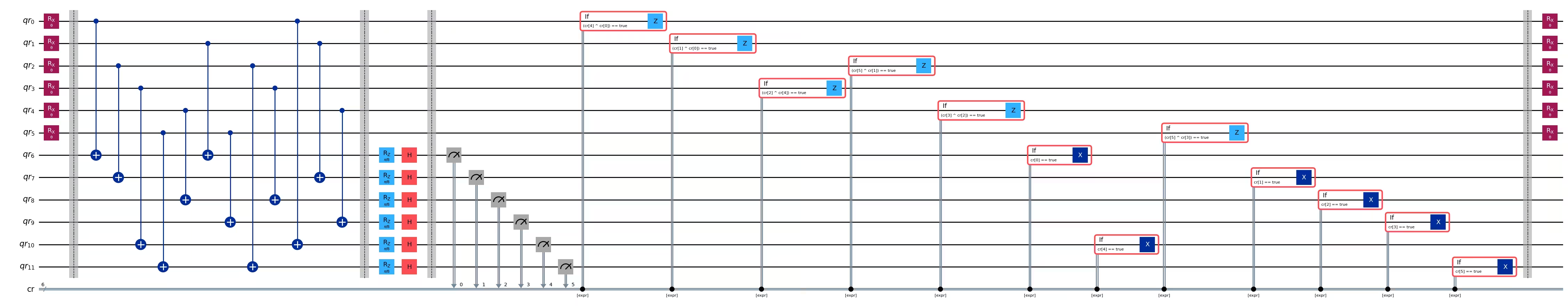
결과로 나타나는 Circuit은 다음과 같습니다:

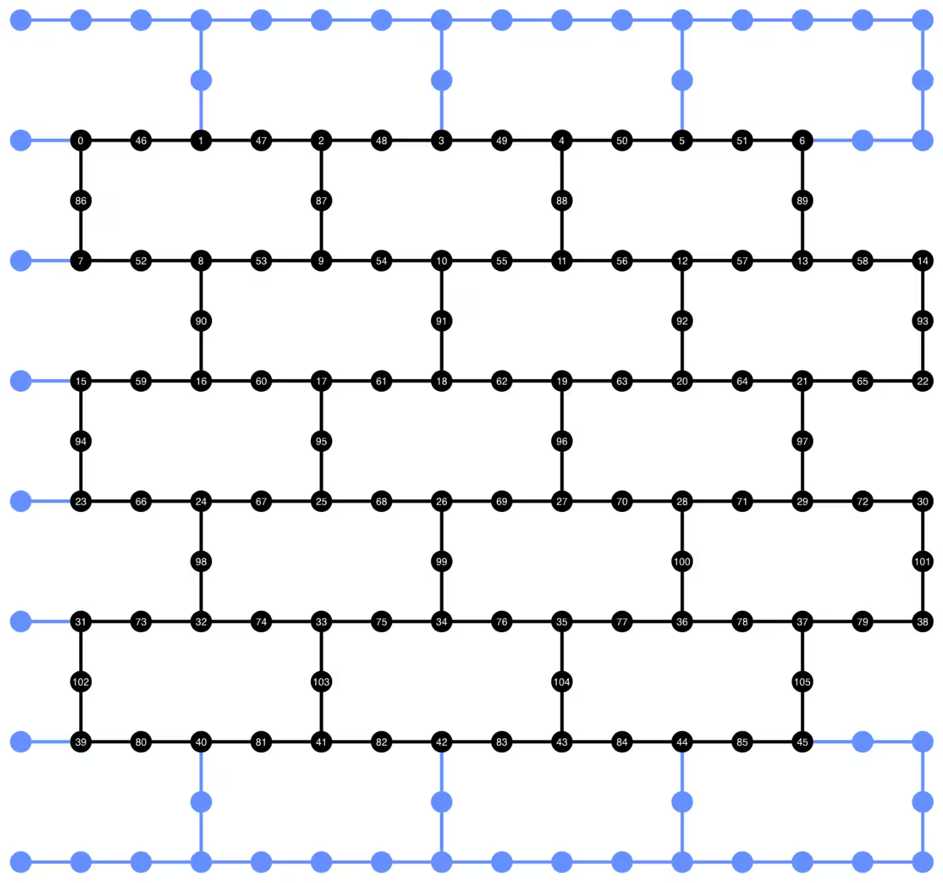
이 접근 방식을 사용하여 벌집 격자를 시뮬레이션하면, 결과 회로는 헤비-헥스 격자를 가진 하드웨어에 완벽하게 내장됩니다. 모든 데이터 큐비트는 육각형 격자를 형성하는 격자의 차수-3 사이트에 위치합니다. 각 데이터 큐비트 쌍은 차수-2 사이트에 위치하는 보조 큐비트를 공유합니다. 아래에서 동적 회로 구현을 위한 큐비트 격자를 구성하며, 보조 큐비트(진한 보라색 원으로 표시)를 도입합니다.

def make_lattice(hex_rows=1, hex_cols=1):
    """Define heavy-hex lattice and corresponding lists of data and ancilla nodes."""
    hex_cmap = CouplingMap.from_hexagonal_lattice(
        hex_rows, hex_cols, bidirectional=False
    )
    data = list(hex_cmap.physical_qubits)

    heavyhex_cmap = CouplingMap()
    for d in data:
        heavyhex_cmap.add_physical_qubit(d)

    # make coupling map
    a = len(data)
    for edge in hex_cmap.get_edges():
        heavyhex_cmap.add_physical_qubit(a)
        heavyhex_cmap.add_edge(edge[0], a)
        heavyhex_cmap.add_edge(edge[1], a)
        a += 1
    ancilla = list(range(len(data), a))
    qubits = data + ancilla

    # color edges
    graph = heavyhex_cmap.graph.to_undirected(multigraph=False)
    edge_colors = rx.graph_misra_gries_edge_color(graph)
    layer_edges = {color: [] for color in edge_colors.values()}
    for edge_index, color in edge_colors.items():
        layer_edges[color].append(graph.edge_list()[edge_index])

    # construct observable
    obs_hex = SparsePauliOp.from_sparse_list(
        [("Z", [i], 1 / len(data)) for i in data],
        num_qubits=len(qubits),
    )

    return (data, qubits, ancilla, layer_edges, heavyhex_cmap, graph, obs_hex)

소규모에서 데이터 큐비트와 보조 큐비트에 대한 헤비-헥스 격자를 시각화합니다:

(data, qubits, ancilla, layer_edges, heavyhex_cmap, graph, obs_hex) = (
    make_lattice(hex_rows=hex_rows, hex_cols=hex_cols)
)

print(f"number of data qubits = {len(data)}")
print(f"number of ancilla qubits = {len(ancilla)}")

node_colors = []
for node in graph.node_indices():
    if node in ancilla:
        node_colors.append("purple")
    else:
        node_colors.append("lightblue")

pos = rx.graph_spring_layout(
    graph,
    k=1 / np.sqrt(len(qubits)),
    repulsive_exponent=2,
    num_iter=200,
)

# Visualize the graph, blue circles are data qubits and purple circles are ancillas
mpl_draw(graph, node_color=node_colors, pos=pos)
plt.show()

number of data qubits = 46
number of ancilla qubits = 60

아래에서 Trotter화된 시간 진화를 위한 동적 회로를 구성합니다. RZZ 게이트는 위에서 설명한 단계를 사용하여 동적 회로 구현으로 대체됩니다.

def gen_hex_dynamic(
    depth=1,
    zz_angle=np.pi / 8,
    θ=Parameter("θ"),
    hex_rows=1,
    hex_cols=1,
    measure=False,
    add_dd=True,
):
    """Build dynamic circuits."""
    (data, qubits, ancilla, layer_edges, heavyhex_cmap, graph, obs_hex) = (
        make_lattice(hex_rows=hex_rows, hex_cols=hex_cols)
    )
    # Initialize circuit
    qr = QuantumRegister(len(qubits), "qr")
    cr = ClassicalRegister(len(ancilla), "cr")
    circuit = QuantumCircuit(qr, cr)

    for k in range(depth):
        # Single-qubit Rx layer
        for d in data:
            circuit.rx(θ, d)
        circuit.barrier()

        # CX gates from data qubits to ancilla qubits
        for same_color_edges in layer_edges.values():
            for e in same_color_edges:
                circuit.cx(e[0], e[1])
        circuit.barrier()

        # Apply Rz rotation on ancilla qubits and rotate into X basis
        for a in ancilla:
            circuit.rz(zz_angle, a)
            circuit.h(a)
        # Add barrier to align terminal measurement
        circuit.barrier()

        # Measure ancilla qubits
        for i, a in enumerate(ancilla):
            circuit.measure(a, i)
        d2ros = {}
        a2ro = {}
        # Retrieve ancilla measurement outcomes
        for a in ancilla:
            a2ro[a] = cr[ancilla.index(a)]

        # For each data qubit, retrieve measurement outcomes of neighboring ancilla qubits
        for d in data:
            ros = [a2ro[a] for a in heavyhex_cmap.neighbors(d)]
            d2ros[d] = ros

        # Build classical feedforward operations (optionally add DD on idling data qubits)
        for d in data:
            if add_dd:
                circuit = add_stretch_dd(circuit, d, f"data_{d}_depth_{k}")

            # # XOR the neighboring readouts of the data qubit; if True, apply Z to it
            ros = d2ros[d]
            parity = ros[0]
            for ro in ros[1:]:
                parity = expr.bit_xor(parity, ro)
            with circuit.if_test(expr.equal(parity, True)):
                circuit.z(d)

        # Reset the ancilla if its readout is 1
        for a in ancilla:
            with circuit.if_test(expr.equal(a2ro[a], True)):
                circuit.x(a)
        circuit.barrier()

    # Final single-qubit Rx layer to match the unitary circuits
    for d in data:
        circuit.rx(θ, d)

    if measure:
        circuit.measure_all()
    return circuit, obs_hex

def add_stretch_dd(qc, q, name):
    """Add XpXm DD sequence."""
    s = qc.add_stretch(name)
    qc.delay(s, q)
    qc.x(q)
    qc.delay(s, q)
    qc.delay(s, q)
    qc.rz(np.pi, q)
    qc.x(q)
    qc.rz(-np.pi, q)
    qc.delay(s, q)
    return qc

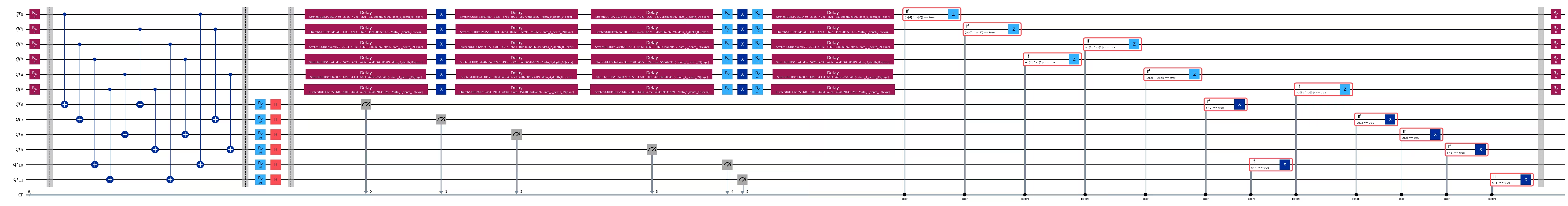
동적 디커플링(DD)과 stretch 지속 시간 지원

ZZ 상호작용을 실현하기 위해 동적 회로 구현을 사용할 때의 한 가지 주의 사항은, 중간 회로 측정과 고전 피드포워드 연산이 일반적으로 양자 게이트보다 실행 시간이 더 길다는 것입니다. 고전 연산이 수행되는 동안 큐비트가 유휴 상태일 때 결어긋남(decoherence)을 억제하기 위해, if_test 문 이전의 데이터 큐비트에 대한 조건부 Z 연산 전, 보조 큐비트의 측정 연산 이후에 동적 디커플링 (DD) 시퀀스를 추가했습니다.

DD 시퀀스는 add_stretch_dd() 함수에 의해 추가되며, 이 함수는 stretch 지속 시간을 사용하여 DD 게이트 사이의 시간 간격을 결정합니다. stretch 지속 시간은 큐비트의 유휴 시간을 채우도록 지연 지속 시간이 늘어날 수 있는 신축적인 시간 지속 시간을 지정하는 방법입니다. stretch로 지정된 지속 시간 변수는 특정 제약 조건을 충족하는 원하는 지속 시간으로 컴파일 시간에 결정됩니다. 이는 DD 시퀀스의 타이밍이 좋은 오류 억제 성능을 달성하는 데 필수적일 때 매우 유용합니다. stretch 타입에 대한 자세한 내용은 OpenQASM 문서를 참조하세요. 현재 Qiskit Runtime에서 stretch 타입에 대한 지원은 실험적입니다. 사용 제약 조건에 대한 자세한 내용은 stretch 문서의 제한 사항 섹션을 참조하세요.

위에서 정의한 함수를 사용하여 DD가 있는 경우와 없는 경우의 Trotter화된 시간 진화 회로와 해당 관측량을 구성합니다. 먼저 소규모 예시의 동적 회로를 시각화합니다:

hex_rows_test = 1
hex_cols_test = 1

(
    data_test,
    qubits_test,
    ancilla_test,
    layer_edges_test,
    heavyhex_cmap_test,
    graph_test,
    obs_hex_test,
) = make_lattice(hex_rows=hex_rows_test, hex_cols=hex_cols_test)

node_colors = []
for node in graph_test.node_indices():
    if node in ancilla_test:
        node_colors.append("purple")
    else:
        node_colors.append("lightblue")
pos = rx.graph_spring_layout(
    graph_test,
    k=5 / np.sqrt(len(qubits_test)),
    repulsive_exponent=2,
    num_iter=150,
)

# display a small example for illustration
node_colors_test = ["lightblue"] * len(graph_test.node_indices())
mpl_draw(graph_test, node_color=node_colors, pos=pos)

circuit_dynamic_test, obs_dynamic_test = gen_hex_dynamic(
    depth=1,
    θ=Parameter("θ"),
    hex_rows=hex_rows_test,
    hex_cols=hex_cols_test,
    measure=False,
    add_dd=False,
)
circuit_dynamic_test.draw("mpl", fold=-1)

circuit_dynamic_dd_test, _ = gen_hex_dynamic(
    depth=1,
    θ=Parameter("θ"),
    hex_rows=hex_rows_test,
    hex_cols=hex_cols_test,
    measure=False,
    add_dd=True,
)
circuit_dynamic_dd_test.draw("mpl", fold=-1)

마찬가지로, 대규모 예시에 대한 동적 회로를 구성합니다:

circuits_dynamic = []
circuits_dynamic_dd = []
observables_dynamic = []
for depth in depths:
    circuit, obs = gen_hex_dynamic(
        depth=depth,
        θ=Parameter("θ"),
        hex_rows=hex_rows,
        hex_cols=hex_cols,
        measure=True,
        add_dd=False,
    )
    circuits_dynamic.append(circuit)

    circuit_dd, _ = gen_hex_dynamic(
        depth=depth,
        θ=Parameter("θ"),
        hex_rows=hex_rows,
        hex_cols=hex_cols,
        measure=True,
        add_dd=True,
    )
    circuits_dynamic_dd.append(circuit_dd)
    observables_dynamic.append(obs)

Step 2: 하드웨어 실행을 위한 문제 최적화

이제 Circuit을 하드웨어에 트랜스파일할 준비가 되었습니다. 유니터리 표준 구현과 동적 Circuit 구현 모두를 하드웨어에 트랜스파일합니다.

하드웨어에 트랜스파일하려면 먼저 Backend를 인스턴스화합니다. 가능한 경우, MidCircuitMeasure (measure_2) 명령어가 지원되는 Backend를 선택합니다.

service = QiskitRuntimeService()
try:
    backend = service.least_busy(
        operational=True,
        simulator=False,
        use_fractional_gates=True,
        filters=lambda b: "measure_2" in b.supported_instructions,
    )
except QiskitBackendNotFoundError:
    backend = service.least_busy(
        operational=True,
        simulator=False,
        use_fractional_gates=True,
    )

동적 Circuit의 트랜스파일

먼저 DD 시퀀스를 추가하는 경우와 추가하지 않는 경우 각각에 대해 동적 Circuit을 트랜스파일합니다. 더 일관된 결과를 위해 모든 Circuit에서 동일한 물리적 Qubit 집합을 사용하도록, 먼저 Circuit을 한 번 트랜스파일한 후 해당 레이아웃을 이후 모든 Circuit에 사용합니다. 이는 패스 매니저의 initial_layout으로 지정됩니다. 그런 다음 Sampler 프리미티브 입력으로 primitive unified blocs(PUB)을 구성합니다.

pm_temp = generate_preset_pass_manager(
    optimization_level=3,
    backend=backend,
)
isa_temp = pm_temp.run(circuits_dynamic[-1])
dynamic_layout = isa_temp.layout.initial_index_layout(filter_ancillas=True)

pm = generate_preset_pass_manager(
    optimization_level=3, backend=backend, initial_layout=dynamic_layout
)

dynamic_isa_circuits = [pm.run(circ) for circ in circuits_dynamic]
dynamic_pubs = [(circ, params) for circ in dynamic_isa_circuits]

dynamic_isa_circuits_dd = [pm.run(circ) for circ in circuits_dynamic_dd]
dynamic_pubs_dd = [(circ, params) for circ in dynamic_isa_circuits_dd]

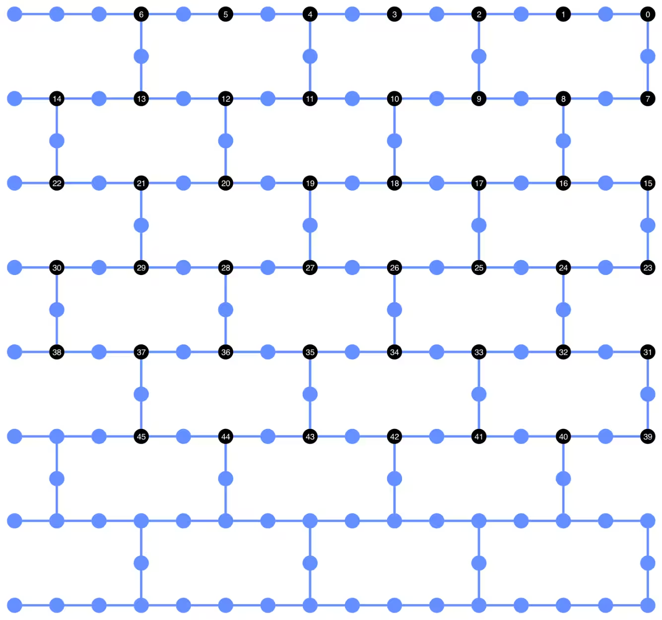
아래에서 트랜스파일된 Circuit의 Qubit 레이아웃을 시각화할 수 있습니다. 검은색 원은 동적 Circuit 구현에 사용된 데이터 Qubit과 앤실라 Qubit을 나타냅니다.

def _heron_coords_r2():
    cord_map = np.array(
        [
            [
                0,
                1,
                2,
                3,
                4,
                5,
                6,
                7,
                8,
                9,
                10,
                11,
                12,
                13,
                14,
                15,
                3,
                7,
                11,
                15,
                0,
                1,
                2,
                3,
                4,
                5,
                6,
                7,
                8,
                9,
                10,
                11,
                12,
                13,
                14,
                15,
                1,
                5,
                9,
                13,
                0,
                1,
                2,
                3,
                4,
                5,
                6,
                7,
                8,
                9,
                10,
                11,
                12,
                13,
                14,
                15,
                3,
                7,
                11,
                15,
                0,
                1,
                2,
                3,
                4,
                5,
                6,
                7,
                8,
                9,
                10,
                11,
                12,
                13,
                14,
                15,
                1,
                5,
                9,
                13,
                0,
                1,
                2,
                3,
                4,
                5,
                6,
                7,
                8,
                9,
                10,
                11,
                12,
                13,
                14,
                15,
                3,
                7,
                11,
                15,
                0,
                1,
                2,
                3,
                4,
                5,
                6,
                7,
                8,
                9,
                10,
                11,
                12,
                13,
                14,
                15,
                1,
                5,
                9,
                13,
                0,
                1,
                2,
                3,
                4,
                5,
                6,
                7,
                8,
                9,
                10,
                11,
                12,
                13,
                14,
                15,
                3,
                7,
                11,
                15,
                0,
                1,
                2,
                3,
                4,
                5,
                6,
                7,
                8,
                9,
                10,
                11,
                12,
                13,
                14,
                15,
            ],
            -1
            * np.array([j for i in range(15) for j in [i] * [16, 4][i % 2]]),
        ],
        dtype=int,
    )

    hcords = []
    ycords = cord_map[0]
    xcords = cord_map[1]
    for i in range(156):
        hcords.append([xcords[i] + 1, np.abs(ycords[i]) + 1])

    return hcords

plot_circuit_layout(
    dynamic_isa_circuits_dd[8],
    backend,
    qubit_coordinates=_heron_coords_r2(),
    view="virtual",
)

참고

plot_circuit_layout()에서 neato를 찾을 수 없다는 오류가 발생하면, graphviz 패키지가 설치되어 있고 PATH에서 사용 가능한지 확인하세요. 기본이 아닌 위치에 설치된 경우(예: MacOS에서 homebrew 사용 시) PATH 환경 변수를 업데이트해야 할 수 있습니다. 이는 다음과 같이 이 노트북 내에서 수행할 수 있습니다:

import os
os.environ['PATH'] = f"path/to/neato{os.pathsep}{os.environ['PATH']}"

dynamic_isa_circuits[1].draw(fold=-1, output="mpl", idle_wires=False)

dynamic_isa_circuits_dd[1].draw(fold=-1, output="mpl", idle_wires=False)

MidCircuitMeasure를 사용한 트랜스파일

MidCircuitMeasure는 중간 Circuit 측정을 수행하기 위해 특별히 보정된 추가 측정 연산입니다. MidCircuitMeasure 명령어는 Backend가 지원하는 measure_2 명령어에 매핑됩니다. measure_2가 모든 Backend에서 지원되는 것은 아닙니다. service.backends(filters=lambda b: "measure_2" in b.supported_instructions)를 사용하여 이를 지원하는 Backend를 찾을 수 있습니다. 여기서는 Backend가 지원하는 경우, Circuit에 정의된 중간 Circuit 측정이 MidCircuitMeasure 연산을 사용하여 실행되도록 Circuit을 트랜스파일하는 방법을 보여줍니다.

아래에서는 measure_2 명령어와 표준 measure 명령어의 지속 시간을 출력합니다.

print(
    f'Mid-circuit measurement `measure_2` duration: {backend.instruction_durations.get('measure_2',0) * backend.dt * 1e9/1e3} μs'
)
print(
    f'Terminal measurement `measure` duration: {backend.instruction_durations.get('measure',0) * backend.dt *1e9/1e3} μs'
)

Mid-circuit measurement `measure_2` duration:  1.624 μs
Terminal measurement `measure` duration: 2.2 μs

"""Pass that replaces terminal measures in the middle of the circuit with
MidCircuitMeasure instructions."""

class ConvertToMidCircuitMeasure(TransformationPass):
    """This pass replaces terminal measures in the middle of the circuit with
    MidCircuitMeasure instructions.
    """

    def __init__(self, target):
        super().__init__()
        self.target = target

    def run(self, dag):
        """Run the pass on a dag."""
        mid_circ_measure = None
        for inst in self.target.instructions:
            if isinstance(inst[0], Instruction) and inst[0].name.startswith(
                "measure_"
            ):
                mid_circ_measure = inst[0]
                break
        if not mid_circ_measure:
            return dag

        final_measure_nodes = calc_final_ops(dag, {"measure"})
        for node in dag.op_nodes(Measure):
            if node not in final_measure_nodes:
                dag.substitute_node(node, mid_circ_measure, inplace=True)

        return dag

pm = PassManager(ConvertToMidCircuitMeasure(backend.target))

dynamic_isa_circuits_meas2 = [pm.run(circ) for circ in dynamic_isa_circuits]
dynamic_pubs_meas2 = [(circ, params) for circ in dynamic_isa_circuits_meas2]

dynamic_isa_circuits_dd_meas2 = [
    pm.run(circ) for circ in dynamic_isa_circuits_dd
]
dynamic_pubs_dd_meas2 = [
    (circ, params) for circ in dynamic_isa_circuits_dd_meas2
]

유니터리 회로의 트랜스파일

동적 회로와 해당 유니터리 대응물 간의 공정한 비교를 위해, 동적 회로에서 사용된 것과 동일한 물리적 Qubit 집합을 데이터 Qubit용 레이아웃으로 사용하여 유니터리 회로를 트랜스파일합니다.

init_layout = [
    dynamic_layout[ind] for ind in range(circuits_unitary[0].num_qubits)
]

pm = generate_preset_pass_manager(
    target=backend.target,
    initial_layout=init_layout,
    optimization_level=3,
)

def transpile_minimize(circ: QuantumCircuit, pm: PassManager, iterations=10):
    """Transpile circuits for specified number of iterations and return the one with smallest two-qubit gate depth"""
    circs = [pm.run(circ) for i in range(iterations)]
    circs_sorted = sorted(
        circs,
        key=lambda x: x.depth(lambda x: x.operation.num_qubits == 2),
    )
    return circs_sorted[0]

unitary_isa_circuits = []
for circ in circuits_unitary:
    circ_t = transpile_minimize(circ, pm, iterations=100)
    unitary_isa_circuits.append(circ_t)

unitary_pubs = [(circ, params) for circ in unitary_isa_circuits]

트랜스파일된 유니터리 회로의 Qubit 레이아웃을 시각화합니다. 검은 원은 유니터리 회로를 트랜스파일하는 데 사용된 물리적 Qubit를 나타내며, 해당 인덱스는 가상 Qubit 인덱스에 대응합니다. 이를 동적 회로의 레이아웃 플롯과 비교하면, 유니터리 회로가 동적 회로의 데이터 Qubit와 동일한 물리적 Qubit 집합을 사용한다는 것을 확인할 수 있습니다.

plot_circuit_layout(
    unitary_isa_circuits[-1],
    backend,
    qubit_coordinates=_heron_coords_r2(),
    view="virtual",
)

이제 트랜스파일된 회로에 DD 시퀀스를 추가하고, 작업 제출을 위한 PUB를 구성합니다.

pm_dd = PassManager(
    [
        ALAPScheduleAnalysis(target=backend.target),
        PadDynamicalDecoupling(
            dd_sequence=[
                XGate(),
                RZGate(np.pi),
                XGate(),
                RZGate(-np.pi),
            ],
            spacing=[1 / 4, 1 / 2, 0, 0, 1 / 4],
            target=backend.target,
        ),
    ]
)

unitary_isa_circuits_dd = pm_dd.run(unitary_isa_circuits)
unitary_pubs_dd = [(circ, params) for circ in unitary_isa_circuits_dd]

유니터리 회로와 동적 회로의 2-Qubit Gate 깊이 비교

# compare circuit depth of unitary and dynamic circuit implementations
unitary_depth = [
    unitary_isa_circuits[i].depth(lambda x: x.operation.num_qubits == 2)
    for i in range(len(unitary_isa_circuits))
]

dynamic_depth = [
    dynamic_isa_circuits[i].depth(lambda x: x.operation.num_qubits == 2)
    for i in range(len(dynamic_isa_circuits))
]

plt.plot(
    list(range(len(unitary_depth))),
    unitary_depth,
    label="unitary circuits",
    color="#be95ff",
)
plt.plot(
    list(range(len(dynamic_depth))),
    dynamic_depth,
    label="dynamic circuits",
    color="#ff7eb6",
)
plt.xlabel("Trotter steps")
plt.ylabel("Two-qubit depth")
plt.legend()

<matplotlib.legend.Legend at 0x374225760>

측정 기반 회로의 주요 장점은, 여러 ZZ 상호작용을 구현할 때 CX 레이어를 병렬화할 수 있고 측정이 동시에 이루어질 수 있다는 점입니다. 이는 모든 ZZ 상호작용이 교환 가능(commute)하기 때문에, 측정 깊이 1로 계산을 수행할 수 있기 때문입니다. 회로를 트랜스파일한 후, 동적 회로 방식이 표준 유니터리 방식보다 2-Qubit 깊이가 훨씬 짧다는 것을 확인할 수 있습니다. 단, 추가적인 중간 회로 측정과 클래식 피드포워드 자체도 시간이 소요되며 고유한 오류 원인을 도입한다는 점은 주의해야 합니다.

Step 3: Qiskit 프리미티브를 사용하여 실행

로컬 테스트 모드

하드웨어에 작업을 제출하기 전에, 로컬 테스트 모드를 사용하여 동적 Circuit의 소규모 시뮬레이션 테스트를 실행할 수 있습니다.

aer_sim = AerSimulator()
pm = generate_preset_pass_manager(backend=aer_sim, optimization_level=1)
circuit_dynamic_test.measure_all()
isa_qc = pm.run(circuit_dynamic_test)
with Batch(backend=aer_sim) as batch:
    sampler = Sampler(mode=batch)
    result = sampler.run([(isa_qc, params)]).result()

print(
    "Simulated average magnetization at trotter step = 1 at three theta values"
)
result[0].data["meas"].expectation_values(obs_dynamic_test[0])

Simulated average magnetization at trotter step = 1 at three theta values

array([ 0.16666667,  0.01855469, -0.13476562])

MPS 시뮬레이션

대규모 Circuit의 경우, matrix_product_state (MPS) 시뮬레이터를 사용할 수 있습니다. 이 시뮬레이터는 선택한 본드 차원에 따라 기댓값에 대한 근사 결과를 제공합니다. 이후 MPS 시뮬레이션 결과를 하드웨어 결과와 비교하기 위한 기준선으로 사용합니다.

# The MPS simulation below took approximately 7 minutes to run on a laptop with Apple M1 chip

mps_backend = AerSimulator(
    method="matrix_product_state",
    matrix_product_state_truncation_threshold=1e-5,
    matrix_product_state_max_bond_dimension=100,
)
mps_sampler = Aer_Sampler.from_backend(mps_backend)

shots = 4096

data_sim = []
for j in range(points):
    circ_list = [
        circ.assign_parameters([params[j]]) for circ in circuits_unitary
    ]

    mps_job = mps_sampler.run(circ_list, shots=shots)
    result = mps_job.result()

    point_data = [
        result[d].data["meas"].expectation_values(observables_unitary)
        for d in depths
    ]

    data_sim.append(point_data)  # data at one theta value

data_sim = np.array(data_sim)

Circuit과 Observable이 준비되었으므로, 이제 Sampler 프리미티브를 사용하여 하드웨어에서 실행합니다.

여기서는 unitary_pubs, dynamic_pubs, dynamic_pubs_dd에 대해 세 개의 작업을 제출합니다. 각각은 세 가지 서로 다른 $\theta$ 파라미터를 가진 아홉 개의 Trotter 단계에 해당하는 파라미터화된 Circuit의 목록입니다.

shots = 10000

with Batch(backend=backend) as batch:
    sampler = Sampler(mode=batch)

    sampler.options.experimental = {
        "execution": {
            "scheduler_timing": True
        },  # set to True to retrieve circuit timing info
    }

    job_unitary = sampler.run(unitary_pubs, shots=shots)
    print(f"unitary: {job_unitary.job_id()}")

    job_unitary_dd = sampler.run(unitary_pubs_dd, shots=shots)
    print(f"unitary_dd: {job_unitary_dd.job_id()}")

    job_dynamic = sampler.run(dynamic_pubs, shots=shots)
    print(f"dynamic: {job_dynamic.job_id()}")

    job_dynamic_dd = sampler.run(dynamic_pubs_dd, shots=shots)
    print(f"dynamic_dd: {job_dynamic_dd.job_id()}")

    job_dynamic_meas2 = sampler.run(dynamic_pubs_meas2, shots=shots)
    print(f"dynamic_meas2: {job_dynamic_meas2.job_id()}")

    job_dynamic_dd_meas2 = sampler.run(dynamic_pubs_dd_meas2, shots=shots)
    print(f"dynamic_dd_meas2: {job_dynamic_dd_meas2.job_id()}")

unitary: d5dtt0ldq8ts73fvbhj0
unitary: d5dtt11smlfc739onuag
dynamic: d5dtt1hsmlfc739onuc0
dynamic_dd: d5dtt25jngic73avdne0
dynamic_meas2: d5dtt2ldq8ts73fvbhm0
dynamic_dd_meas2: d5dtt2tjngic73avdnf0

Step 4: 결과를 후처리하여 원하는 고전 형식으로 반환

작업이 완료된 후, 작업 결과 메타데이터에서 Circuit 실행 시간을 가져와 Circuit 스케줄 정보를 시각화할 수 있습니다. Circuit의 스케줄링 정보를 시각화하는 방법에 대한 자세한 내용은 이 페이지를 참조하세요.

# Circuit durations is reported in the unit of `dt` which can be retrieved from `Backend` object
unitary_durations = [
    job_unitary.result()[i].metadata["compilation"]["scheduler_timing"][
        "circuit_duration"
    ]
    for i in depths
]

dynamic_durations = [
    job_dynamic.result()[i].metadata["compilation"]["scheduler_timing"][
        "circuit_duration"
    ]
    for i in depths
]

dynamic_durations_meas2 = [
    job_dynamic_meas2.result()[i].metadata["compilation"]["scheduler_timing"][
        "circuit_duration"
    ]
    for i in depths
]

result_dd = job_dynamic_dd.result()[1]
circuit_schedule_dd = result_dd.metadata["compilation"]["scheduler_timing"][
    "timing"
]

# to visualize the circuit schedule, one can show the figure below
fig_dd = draw_circuit_schedule_timing(
    circuit_schedule=circuit_schedule_dd,
    included_channels=None,
    filter_readout_channels=False,
    filter_barriers=False,
    width=1000,
)

# Save to a file since the figure is large
fig_dd.write_html("scheduler_timing_dd.html")

아래에서 유니터리 Circuit과 동적 Circuit의 Circuit 실행 시간을 플롯합니다. 아래 플롯에서, 중간 Circuit 측정과 고전 연산에 필요한 시간에도 불구하고, measure_2를 사용한 동적 Circuit 구현이 유니터리 구현과 비슷한 Circuit 실행 시간을 보임을 확인할 수 있습니다.

# visualize circuit durations

def convert_dt_to_microseconds(circ_duration: List, backend_dt: float):
    dt = backend_dt * 1e6  # dt in microseconds
    return list(map(lambda x: x * dt, circ_duration))

dt = backend.target.dt
plt.plot(
    depths,
    convert_dt_to_microseconds(unitary_durations, dt),
    color="#be95ff",
    linestyle=":",
    label="unitary",
)
plt.plot(
    depths,
    convert_dt_to_microseconds(dynamic_durations, dt),
    color="#ff7eb6",
    linestyle="-.",
    label="dynamic",
)
plt.plot(
    depths,
    convert_dt_to_microseconds(dynamic_durations_meas2, dt),
    color="#ff7eb6",
    linestyle="-.",
    marker="s",
    mfc="none",
    label="dynamic w/ meas2",
)

plt.xlabel("Trotter steps")
plt.ylabel(r"Circuit durations in $\mu$s")
plt.legend()

<matplotlib.legend.Legend at 0x17f73c6e0>

작업이 완료된 후, 아래에서 데이터를 가져와 앞서 구성한 Observable observables_unitary 또는 observables_dynamic으로 추정한 평균 자기화를 계산합니다.

runs = {
    "unitary": (
        job_unitary,
        [observables_unitary] * len(circuits_unitary),
    ),
    "unitary_dd": (
        job_unitary_dd,
        [observables_unitary] * len(circuits_unitary),
    ),
    # Omitting Dyn w/o DD and Dynamic w/ DD plots for better readability
    # "dynamic": (job_dynamic, observables_dynamic),
    # "dynamic_dd": (job_dynamic_dd, observables_dynamic),
    "dynamic_meas2": (job_dynamic_meas2, observables_dynamic),
    "dynamic_dd_meas2": (
        job_dynamic_dd_meas2,
        observables_dynamic,
    ),
}

data_dict = {}
for key, (job, obs) in runs.items():
    data = []
    for i in range(points):
        data.append(
            [
                job.result()[ind].data["meas"].expectation_values(obs[ind])[i]
                for ind in depths
            ]
        )
    data_dict[key] = data

아래에서는 서로 다른 $\theta$ 값(국소 자기장의 세기에 해당)에 따른 Trotter 단계의 함수로서 스핀 자기화를 플롯합니다. 유니터리 이상 Circuit에 대한 사전 계산된 MPS 시뮬레이션 결과와 다음의 실험 결과를 함께 플롯합니다:

1. DD를 적용한 유니터리 Circuit 실행
2. DD와 MidCircuitMeasure를 적용한 동적 Circuit 실행

plt.figure(figsize=(10, 6))

colors = ["#0f62fe", "#be95ff", "#ff7eb6"]
for i in range(points):
    plt.plot(
        depths,
        data_sim[i],
        color=colors[i],
        linestyle="solid",
        label=f"θ={pi_check(i*max_angle/(points-1))} (MPS)",
    )
    # plt.plot(
    #     depths,
    #     data_dict["unitary"][i],
    #     color=colors[i],
    #     linestyle=":",
    #     label=f"θ={pi_check(i*max_angle/(points-1))} (Unitary)",
    # )

    plt.plot(
        depths,
        data_dict["unitary_dd"][i],
        color=colors[i],
        marker="o",
        mfc="none",
        linestyle=":",
        label=f"θ={pi_check(i*max_angle/(points-1))} (Unitary w/DD)",
    )

    # Omitting Dyn w/o DD and Dynamic w/ DD plots for better readability
    # plt.plot(
    #     depths,
    #     data_dict["dynamic"][i],
    #     color=colors[i],
    #     linestyle="-.",
    #     label=f"θ={pi_check(i*max_angle/(points-1))} (Dyn w/o DD)",
    # )
    # plt.plot(
    #     depths,
    #     data_dict["dynamic_dd"][i],
    #     marker="D",
    #     mfc="none",
    #     color=colors[i],
    #     linestyle="-.",
    #     label=f"θ={pi_check(i*max_angle/(points-1))} (Dynamic w/ DD)",
    # )

    # plt.plot(
    #     depths,
    #     data_dict["dynamic_meas2"][i],
    #     color=colors[i],
    #     marker="s",
    #     mfc="none",
    #     linestyle=':',
    #     label=f"θ={pi_check(i*max_angle/(points-1))} (Dynamic w/ MidCircuitMeas)",
    # )

    plt.plot(
        depths,
        data_dict["dynamic_dd_meas2"][i],
        color=colors[i],
        marker="*",
        markersize=8,
        linestyle=":",
        label=f"θ={pi_check(i*max_angle/(points-1))} (Dynamic w/ DD & MidCircuitMeas)",
    )

plt.xlabel("Trotter steps", fontsize=16)
plt.ylabel("Average magnetization", fontsize=16)
plt.xticks(rotation=45)
handles, labels = plt.gca().get_legend_handles_labels()
plt.legend(
    handles,
    labels,
    loc="upper right",
    bbox_to_anchor=(1.46, 1.0),
    shadow=True,
    ncol=1,
)
plt.title(
    f"{hex_rows}x{hex_cols} hex ring, {num_qubits} data qubits, {len(ancilla)} ancilla qubits \n{backend.name}: Sampler"
)
plt.show()

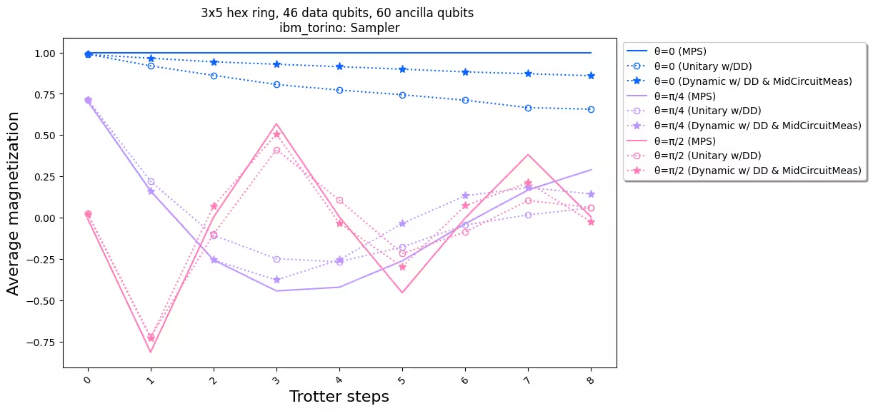
실험 결과를 시뮬레이션과 비교해보면, 동적 Circuit 구현(별표 점선)이 전반적으로 표준 유니터리 구현(원형 점선)보다 성능이 우수함을 확인할 수 있습니다. 요약하면, 우리는 하드웨어의 네이티브 토폴로지가 아닌 허니컴 격자의 이징 스핀 모델을 시뮬레이션하기 위한 해결책으로 동적 Circuit을 제시합니다. 동적 Circuit 솔루션은 SWAP Gate 사용보다 짧은 2-Qubit Gate 깊이로 최근접 이웃이 아닌 Qubit 간의 ZZ 상호작용을 가능하게 하며, 그 대신 추가적인 앙실라 Qubit와 고전 피드포워드 연산을 도입합니다.

참고 문헌

[1] Quantum computing with Qiskit, by Javadi-Abhari, A., Treinish, M., Krsulich, K., Wood, C.J., Lishman, J., Gacon, J., Martiel, S., Nation, P.D., Bishop, L.S., Cross, A.W. and Johnson, B.R., 2024. arXiv preprint arXiv:2405.08810 (2024)