Kipu Quantum의 Rimay 양자 특성 추출로 신용 위험 분류하기
Qiskit Functions는 IBM Quantum® Premium Plan, Flex Plan, On-Prem(IBM Quantum Platform API 경유) Plan 사용자에게만 제공되는 실험적 기능입니다. 프리뷰 릴리스 상태이며 변경될 수 있습니다.
사용량 추정: Nighthawk r2 프로세서에서 2분. (참고: 이는 추정치일 뿐이며 실제 실행 시간은 다를 수 있습니다.)
학습 목표
-
범주형 열과 수치형 열이 있는 표 형식 데이터를 Rimay Qiskit Function용으로 준비합니다.
-
학습 데이터로 양자 특성 매핑을 피팅하고 같은 실행에서 테스트 데이터를 매핑합니다.
-
양자 변환 특성만 사용한 경우와 원래 특성과 결합한 경우로 나누어 고전 모델을 학습합니다.
-
결과를 순수 고전 기준선과 비교합니다.
사전 요구 사항
이 튜토리얼을 시작하기 전에 다음 주제에 익숙해야 합니다.
-
scikit-learn을 이용한 지도 분류
배경
산업 분야의 많은 머신러닝 문제는 소규모 또는 중규모의 표 형식 데이터셋을 다루며, 여기서는 데이터를 더 추가할 수 없고 모델 정확도가 정체됩니다. 신용 위험 평가가 대표적인 예입니다. 대출 기관은 수십 개의 속성을 사용하여 신청자가 신용을 상환할 가능성이 있는지 판단합니다.
Kipu Quantum의 Qiskit Function인 Rimay는 이러한 파이프라인에 양자 전처리 단계를 추가합니다. 이는 디지털화된 반단열(counterdiabatic) 양자 특성 추출 알고리즘 [1]을 구현합니다. 모든 입력 특성은 하나의 큐비트에 매핑됩니다. 특성 값과 특성 간 상호 정보량이 스핀 글래스 해밀토니안의 국소 장과 결합을 정합니다. 그런 다음 반단열 동역학이 양자 시스템을 저에너지 상태로 발전시키며, 마지막에 측정한 단일체 및 이체 기댓값이 새로운 양자 변환 특성이 됩니다. 이러한 특성은 입력 사이의 비선형 상관관계를 포착하며, 어떤 고전 모델에도 입력할 수 있습니다.
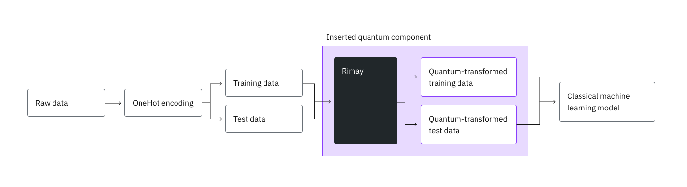
이 튜토리얼에서는 OpenML [2]의 독일 신용 데이터셋(신청자 1000명, 속성 20개)을 사용하여 랜덤 포레스트 분류기를 학습합니다. 먼저 고전 기준선을 설정하고, 데이터를 Rimay로 보낸 다음, 마지막으로 양자 변환 특성만 사용한 경우와 원래 특성과 결합한 경우에 대해 같은 종류의 모델을 학습합니다.
요구 사항
이 튜토리얼을 시작하기 전에 다음 패키지가 설치되어 있는지 확인하세요.
-
IBM Quantum Compute 클라이언트(
pip install qiskit-ibm-runtime) -
Qiskit Functions(
pip install qiskit-ibm-catalog) -
scikit-learn(
pip install scikit-learn) -
pandas (
pip install pandas) -
Matplotlib (
pip install matplotlib)
Qiskit Functions Catalog의 Rimay 함수에도 접근할 수 있어야 합니다.
설정
패키지를 가져오고 두 가지 도우미 함수를 정의합니다. 하나는 랜덤 포레스트를 학습하는 함수이고, 다른 하나는 튜토리얼 전반에서 사용하는 지표를 계산하는 함수입니다.
# Added by doQumentation — installs the packages this notebook needs if they are missing
import importlib.util

_needed = {"matplotlib": "matplotlib", "numpy": "numpy", "pandas": "pandas", "qiskit_ibm_catalog": "qiskit-ibm-catalog", "sklearn": "scikit-learn"}
_missing = [pip for module, pip in _needed.items()
            if importlib.util.find_spec(module) is None]
# One at a time, so a package that fails to install does not block the others
for _pip in _missing:
    %pip install -q {_pip}
if not _missing:
    print("\u2713 All required packages are installed")
import matplotlib.pyplot as plt
import numpy as np
import pandas as pd
from qiskit_ibm_catalog import QiskitFunctionsCatalog
from sklearn.datasets import fetch_openml
from sklearn.ensemble import RandomForestClassifier
from sklearn.metrics import (
    accuracy_score,
    f1_score,
    precision_score,
    recall_score,
    roc_auc_score,
)
from sklearn.model_selection import train_test_split
from sklearn.preprocessing import OneHotEncoder

def train_random_forest(x, y, n_estimators, max_depth):
    """Train a random forest classifier with fixed hyperparameters."""
    model = RandomForestClassifier(
        n_estimators=n_estimators,
        max_depth=max_depth,
        min_samples_split=5,
        min_samples_leaf=1,
        max_features="sqrt",
        random_state=42,
        n_jobs=-1,
    )
    return model.fit(x, y)

def evaluate(model, x, y):
    """Return the classification metrics of a trained model on a test set."""
    y_pred = model.predict(x)
    y_proba = model.predict_proba(x)[:, 1]
    return {
        "Accuracy": accuracy_score(y, y_pred),
        "AUC": roc_auc_score(y, y_proba),
        "F1 score": f1_score(y, y_pred),
        "Precision": precision_score(y, y_pred),
        "Recall": recall_score(y, y_pred),
    }
IBM Quantum 자격 증명 구성
IBM Quantum Platform API 키로 인증하고, Rimay 함수를 로드한 다음, 인스턴스에서 사용할 수 있는 가장 한가한 양자 프로세서를 선택합니다.
catalog = QiskitFunctionsCatalog(channel="ibm_quantum_platform")
rimay = catalog.load("kipu-quantum/rimay")

backend = catalog.least_busy(operational=True, simulator=False)
print(backend.name, backend.num_qubits)
ibm_fez 156
1단계: 고전 입력을 양자 문제로 매핑하기
Rimay는 모든 수치형 입력 특성을 하나의 큐비트에 매핑하므로, 첫 단계는 원시 표를 수치형 특성으로 바꾸는 것입니다.
데이터셋 로드
OpenML에서 German credit 데이터셋을 직접 불러옵니다. class 열에는 레이블이 들어 있으며, 대출을 상환한 신청자는 good, 상환하지 않은 신청자는 bad입니다.
df = fetch_openml(data_id=31, as_frame=True).frame
print(df.shape)
df.head()
(1000, 21)
checking_status  duration                  credit_history  \
0              <0         6  critical/other existing credit
1        0<=X<200        48                   existing paid
2     no checking        12  critical/other existing credit
3              <0        42                   existing paid
4              <0        24              delayed previously

               purpose  credit_amount    savings_status employment  \
0             radio/tv           1169  no known savings        >=7
1             radio/tv           5951              <100     1<=X<4
2            education           2096              <100     4<=X<7
3  furniture/equipment           7882              <100     4<=X<7
4              new car           4870              <100     1<=X<4

   installment_commitment     personal_status other_parties  ...  \
0                       4         male single          none  ...
1                       2  female div/dep/mar          none  ...
2                       2         male single          none  ...
3                       2         male single     guarantor  ...
4                       3         male single          none  ...

   property_magnitude age  other_payment_plans   housing existing_credits  \
0         real estate  67                 none       own                2
1         real estate  22                 none       own                1
2         real estate  49                 none       own                1
3      life insurance  45                 none  for free                1
4   no known property  53                 none  for free                2

                  job num_dependents  own_telephone foreign_worker class
0             skilled              1            yes            yes  good
1             skilled              1           none            yes   bad
2  unskilled resident              2           none            yes  good
3             skilled              2           none            yes  good
4             skilled              2           none            yes   bad

[5 rows x 21 columns]
특성 인코딩
레이블을 이진 값으로 변환하고, 13개의 범주형 열을 원-핫 인코딩합니다. 이 코드는 중복되는 특성을 피하기 위해 각 열의 첫 번째 범주를 제거하며, 그 결과 48개의 수치형 특성이 만들어집니다.
y = (df["class"] == "good").astype(int)

features = df.drop(columns="class")
categorical_cols = [
    col for col in features.columns if features[col].dtype.name == "category"
]
encoder = OneHotEncoder(
    sparse_output=False, handle_unknown="ignore", drop="first"
)
encoded = pd.DataFrame(
    encoder.fit_transform(features[categorical_cols]),
    columns=encoder.get_feature_names_out(categorical_cols),
    index=features.index,
)
x = pd.concat([features.drop(columns=categorical_cols), encoded], axis=1)
print(f"{x.shape[1]} features")
48 features
학습 세트와 테스트 세트로 분할
신청자의 20%를 테스트 세트로 따로 떼어 둡니다. 층화 분할을 사용하면 두 세트에서 good 신용과 bad 신용의 비율이 같게 유지됩니다.
x_train, x_test, y_train, y_test = train_test_split(
    x, y, test_size=0.2, random_state=42, stratify=y
)
print(f"Training set: {x_train.shape}, test set: {x_test.shape}")
Training set: (800, 48), test set: (200, 48)
고전적 기준선 설정
고전적 특성으로 랜덤 포레스트를 학습시킵니다. 4단계에서 양자 변환 특성의 지표를 이 모델의 지표와 비교합니다.
baseline = train_random_forest(
    x_train, y_train, n_estimators=500, max_depth=12
)
results = {"Classical": evaluate(baseline, x_test, y_test)}
pd.DataFrame(results).T
Accuracy       AUC  F1 score  Precision    Recall
Classical     0.765  0.781071  0.845902   0.781818  0.921429
데이터를 Rimay에 업로드
Rimay는 함수에 업로드한 CSV 파일에서 입력을 읽습니다. 특성과 레이블은 서로 다른 파일에 넣습니다. 테스트 세트도 함께 업로드하면, Rimay가 학습 세트로 맞춘(fit) 것과 동일한 매핑으로 테스트 세트를 변환합니다.
x_train.to_csv("x_train.csv", index=False)
y_train.to_csv("y_train.csv", index=False)
x_test.to_csv("x_test.csv", index=False)

for file_name in ("x_train.csv", "y_train.csv", "x_test.csv"):
    catalog.file_upload(file_name, rimay)
2단계: 양자 하드웨어 실행에 맞게 문제 최적화
Rimay는 선택한 프로세서에 맞게 회로를 구성하고 트랜스파일하므로, 직접 최적화할 회로가 없습니다. 다음 제약 조건 안에서 회로당 샷 수를 지정합니다.
-
모든 특성에는 큐비트가 하나씩 필요하므로, 프로세서의 큐비트 수는 데이터셋의 특성 수 이상이어야 합니다.
-
Rimay는 학습 행과 테스트 행을 합쳐 행마다 회로 하나를 실행합니다. 하나의 작업은 최대 1,000만 번까지 실행을 요청할 수 있으므로, 행 수에
shots를 곱한 값이 이 한도 안에 있어야 합니다.
작업을 제출하기 전에 두 한도를 모두 확인하세요.
작업은 회로가 대기열에서 기다리는 시간을 포함해 24시간 안에 끝나야 하며, 그렇지 않으면 결과 없이 중단됩니다.
shots = 5000

n_rows = len(x_train) + len(x_test)
n_features = x_train.shape[1]
print(f"Qubits needed: {n_features} of {backend.num_qubits} available")
print(f"Executions: {n_rows * shots:,} of 10,000,000 allowed")
Qubits needed: 48 of 156 available
Executions: 5,000,000 of 10,000,000 allowed
함수 크기 계산
모든 작업은 S, M, L 중 하나의 함수 크기로 실행되며, 이 크기가 작업이 실행될 컴퓨팅 리소스를 결정합니다. Rimay에서는 작업이 매핑하는 행 수(학습 행과 테스트 행의 합)에 따라 크기가 달라집니다. 너무 작은 크기를 요청하면 작업이 오류 4600으로 실패합니다. 각 크기와 한도는 Rimay 가이드의 함수 크기를 참조하세요.
다음 셀은 크기 계산기를 정의합니다. 이 계산기는 사용자의 컴퓨터에서 실행되며, 전달된 데이터만 읽고 아무것도 제출하지 않습니다.
from os import PathLike
from typing import Any, Literal, Sequence, Sized

Size = Literal["S", "M", "L"]

# Upper bounds (inclusive) in samples.
_SMALL = 2_999
_MEDIUM = 9_999

FIT_TRANSFORM, TRANSFORM, DELETE = "fit-transform", "transform", "delete"

# Which positions of input_file hold samples, per mode. The labels in
# y_train submit no circuits of their own, so they are not counted.
SAMPLE_POSITIONS = {FIT_TRANSFORM: (0, 2), TRANSFORM: (0,)}

def calculate_function_size(problem: Sequence[Sized], **kwargs: Any) -> Size:
    """Return the size ("S", "M" or "L") required to run the function."""
    metrics = _measure(problem, **kwargs)
    if _is_small(metrics):
        return "S"
    if _is_medium(metrics):
        return "M"
    return "L"

def _measure(problem: Sequence[Sized], **kwargs: Any) -> dict:
    """The samples the job submits."""
    return {"samples": count_samples(problem, kwargs.get("mode"))}

def count_samples(problem: Sequence[Sized], mode: Any) -> int:
    """Rows across the data sets of ``problem`` that carry samples."""
    if mode == DELETE:
        return 0
    if mode not in SAMPLE_POSITIONS:
        raise ValueError(f"cannot size mode {mode!r}")
    if _is_name(problem) or (
        isinstance(problem, (list, tuple))
        and any(_is_name(data) for data in problem)
    ):
        raise TypeError(
            "pass the data, not the file name: read each input_file, e.g. with "
            "pandas.read_csv, and pass the data sets in input_file order"
        )
    if not isinstance(problem, (list, tuple)):
        raise TypeError(
            "pass a list of data sets in input_file order, e.g. [x_train, y_train], "
            f"not a single {type(problem).__name__}"
        )
    return sum(
        len(problem[i]) for i in SAMPLE_POSITIONS[mode] if i < len(problem)
    )

def _is_name(value: Any) -> bool:
    """A file name or path rather than data."""
    return isinstance(value, (str, bytes, PathLike))

def _is_small(metrics: dict) -> bool:
    """Determine if the metrics fit T-size 'S'."""
    return metrics["samples"] <= _SMALL

def _is_medium(metrics: dict) -> bool:
    """Determine if the metrics fit T-size 'M'."""
    return metrics["samples"] <= _MEDIUM
실행 모드와 함께, input_file에 있는 파일과 같은 순서로 데이터 세트를 전달합니다.
size = calculate_function_size(
    [x_train, y_train, x_test], mode="fit-transform"
)
print(size)
S
3단계: Qiskit 프리미티브를 사용하여 실행
Rimay를 fit-transform 모드로 실행합니다. 이 모드는 x_train.csv와 y_train.csv로 양자 특성 매핑을 맞추고(fit), 그 매핑으로 학습 세트와 테스트 세트를 모두 변환합니다. input_file에 있는 파일의 순서가 중요합니다. 학습 특성, 학습 레이블, 그리고 선택 사항인 테스트 특성 순으로 나열하세요. 계산한 크기를 function_size로 전달합니다.
job = rimay.run(
    mode="fit-transform",
    input_file=[
        "x_train.csv",
        "y_train.csv",
        "x_test.csv",
    ],  # This order matters
    backend_name=backend.name,
    shots=shots,
    function_size=size,
)
print(job.job_id)
de5094df-bb17-4924-9605-d6196a4aa999
작업 모니터링
작업이 실행되는 동안 상태를 확인합니다. job.result()는 작업이 끝날 때까지 대기(block)합니다.
print(job.status())
INITIALIZING
result = job.result()
print(result["output_files"])
['de5094df-bb17-4924-9605-d6196a4aa999_xq_train.csv', 'de5094df-bb17-4924-9605-d6196a4aa999_xq_test.csv']
결과에는 이번 실행에서 맞춘 매핑을 식별하는 mapping_id가 들어 있습니다. 이 튜토리얼에서는 같은 실행에서 테스트 세트를 이미 변환했으므로 이 ID가 필요하지 않습니다. 나중에 mode="transform"으로 새 행을 변환하려면 이 ID를 기록해 두세요. 맞춘 매핑에 접근하는 유일한 방법이며, ID가 없으면 새 매핑을 다시 맞추고 비용도 다시 지불해야 합니다. 이 매핑은 해당 프로세서의 큐비트 레이아웃에 맞게 만들어지므로, 이후의 transform 실행에서도 같은 backend_name을 전달해야 합니다.
mapping_id = result["mapping_id"]
4단계: 후처리하여 원하는 고전적 형식으로 결과 반환
양자 변환 특성 다운로드
output_files에 있는 이름을 사용하여 작업이 기록한 파일을 다운로드합니다. 각 이름은 작업 ID로 시작하므로, 이번 실행의 파일은 이후 실행 뒤에도 그대로 남아 있습니다. 각 파일이 자신의 이름으로 저장되도록 target_name을 전달하세요.
train_file, test_file = result["output_files"]
for file_name in (train_file, test_file):
    catalog.file_download(file_name, rimay, target_name=file_name)

xq_train = pd.read_csv(train_file).to_numpy()
xq_test = pd.read_csv(test_file).to_numpy()
print(f"Quantum-transformed features: {xq_train.shape[1]}")
586kiB [00:00, 1.13MiB/s]
147kiB [00:00, 336kiB/s]
Quantum-transformed features: 99
양자 변환 특성으로 학습
양자 변환 특성만으로 랜덤 포레스트를 학습시킵니다.
quantum = train_random_forest(
    xq_train, y_train, n_estimators=900, max_depth=15
)
results["Quantum"] = evaluate(quantum, xq_test, y_test)
고전적 특성과 양자 특성을 결합하여 학습
원래 특성과 양자 변환 특성을 쌓아 합친 다음, 그 조합으로 동일한 모델을 학습시킵니다.
xh_train = np.hstack([x_train.to_numpy(), xq_train])
xh_test = np.hstack([x_test.to_numpy(), xq_test])

hybrid = train_random_forest(
    xh_train, y_train, n_estimators=900, max_depth=15
)
results["Hybrid"] = evaluate(hybrid, xh_test, y_test)
결과 비교
테스트 세트에서 세 모델을 비교합니다.
comparison = pd.DataFrame(results).T
print(comparison.round(3))

comparison[["Accuracy", "AUC", "F1 score"]].T.plot.bar(rot=0, figsize=(8, 4))
plt.ylim(0.5, 1.0)
plt.ylabel("Score on the test set")
plt.title("Random forest on classical, quantum, and hybrid features")
plt.show()
Accuracy    AUC  F1 score  Precision  Recall
Classical     0.765  0.781     0.846      0.782   0.921
Quantum       0.730  0.784     0.827      0.750   0.921
Hybrid        0.730  0.791     0.825      0.756   0.907

AUC는 결정 임계값과 무관하게 모델이 good 신용을 bad 신용보다 얼마나 잘 높게 순위 매기는지를 측정하므로, 불균형한 이 데이터셋(good 신용 70%)에서 가장 유용한 지표입니다. Kipu Quantum의 벤치마크에서 양자 변환 특성만으로는 고전적 기준선과 비슷한 AUC에 도달했고, 둘을 결합한 하이브리드 모델은 가장 높은 AUC와 F1 점수에 도달했습니다. 따라서 양자 변환 특성은 고전적 특성만으로는 얻을 수 없는 정보를 추가합니다.
정리(선택 사항)
맞춘 매핑은 삭제하기 전까지 계속 사용할 수 있습니다. 이 매핑으로 더 이상 데이터를 변환하지 않으려면 삭제하세요. 삭제는 양자 연산을 수행하지 않고 QPU 시간도 사용하지 않으며, 되돌릴 수 없습니다.
# rimay.run(mode="delete", mapping_id=mapping_id).result()
{'output_files': [],
 'mode': 'delete',
 'deleted': True,
 'mapping_id': 'eUCy4EnZM7G9jYo5b2Pu-TuCXK7zX_wPTT67g9J1dVE',
 'metadata': {'version': '0.6.0', 'resource_usage': {}}}
결론
달성한 내용
이 튜토리얼에서 다음을 달성했습니다.
-
범주형 및 수치형 속성이 있는 실제 신용 위험 데이터셋을 양자 특성 추출을 위해 준비했습니다.
-
고전적 랜덤 포레스트 기준선을 설정했습니다.
-
Rimay를 사용하여 양자 하드웨어에서 양자 특성 매핑을 맞추고, 학습 세트와 테스트 세트를 한 번의 실행으로 변환했습니다.
-
양자 변환 특성과 결합 특성으로 동일한 모델을 학습시키고 기준선과 비교했습니다.
핵심 요점
-
Rimay는 추가 전처리 단계 하나로 기존 머신러닝 파이프라인에 들어맞습니다. 데이터 준비 과정과 고전적 모델은 그대로 유지합니다.
-
큐비트 수는 입력 특성의 수를 제한하고, 행 수에
shots를 곱한 값은 단일 작업의 크기를 제한합니다. -
모델이 둘 다 활용할 수 있으므로, 기본적으로 양자 변환 특성을 원래 특성과 결합하여 사용하세요.
다음 단계
참고 문헌
[1] Simen, A., et al. (2025). Digitized Counterdiabatic Quantum Feature Extraction. arXiv preprint arXiv:2510.13807.
[2] Hofmann, H. (1994). Statlog (German Credit Data). OpenML dataset 31.
[3] Zhang, Q., et al. (2026). Quantum-enhanced satellite image classification. arXiv preprint arXiv:2602.18350.