양자 근사 다목적 최적화

사용량 추정: Heron r2 프로세서에서 10분 (참고: 추정치일 뿐이며 실제 실행 시간은 다를 수 있습니다.)

학습 목표

이 튜토리얼에서는 기수 제약이 있는 포트폴리오 최적화 문제를 풉니다. 정확히 $K$개의 자산을 보유해야 한다는 제약 하에서 위험, 수익, 분산 목표의 균형을 맞춰 최적 포트폴리오의 집합을 찾습니다.

이 튜토리얼을 마치면 다음을 이해하게 됩니다.

• 서로 상충하는 세 가지 목표, 즉 낮은 위험, 높은 수익, 좋은 분산을 가진 포트폴리오 선택 문제를 양자 최적화 문제로 표현하는 방법.

• 목적 가중치 집합에 걸쳐 단일 QAOA 회로를 훑어 최적의 절충 포트폴리오로 이루어진 파레토 프런티어를 그려내는 방법.

• XY 믹서가 탐색을 "정확히 K개의 자산을 고르는" 부분공간 안에 머물게 하여, 페널티 항이 필요 없고 측정된 비트열을 사후 선택하는 것만으로 실현 가능성이 보장되는 방법.

• 정확히 최적화하기에는 너무 큰 규모에서 행렬곱상태 시뮬레이터로 회로의 각도를 학습시키는 방법. Kotil 등(arXiv:2503.22797)의 방식을 따릅니다.

사전 지식

다음 내용에 익숙하면 좋습니다.

• Qiskit 패턴 워크플로(매핑, 최적화, 실행, 후처리).

• QAOA의 기초.

배경

포트폴리오 매니저는 숫자 하나만 최적화하는 경우가 드뭅니다. 수익은 높고, 위험(그 수익의 분산)은 낮기를 원하며, 보유 자산이 여러 섹터에 퍼져 있어 시장의 어느 한 부분에 과도하게 노출되지 않기를 바랍니다. 이 목표들은 서로 충돌합니다. 수익이 가장 높은 자산은 변동성도 가장 큰 경우가 많고, 한 인기 섹터에 집중하면 분산 효과가 떨어집니다.

유일한 "최고" 포트폴리오는 없습니다. 대신 파레토 프런티어가 있습니다. 한 목표를 개선하려면 다른 목표를 포기해야 하는 포트폴리오들의 집합입니다. 우리의 목표는 이 프런티어를 그려서 의사결정자가 선호하는 절충안을 고를 수 있게 하는 것입니다.

문제를 $N$개 중 정확히 $K$개의 자산을 고르는 것으로 설정합니다(각 자산은 포함되거나 제외되며, 자산당 큐비트 하나). 세 개의 해밀토니안이 세 가지 목표를 인코딩합니다. 이들을 단체(simplex) 위에 놓인(합이 1인) 가중치 $c$로 결합하고, QAOA Sampler가 각 가중치 선택에 대해 좋은 포트폴리오를 반환합니다. 가중치를 훑으면 위험 대 수익 대 분산의 상대적 중요도가 훑어지고, 샘플링된 모든 포트폴리오의 합집합이 파레토 프런티어를 그립니다.

먼저 브루트 포스로 검증할 수 있는 작은 8개 자산 예제로 전체 워크플로를 살펴본 다음, 양자 하드웨어에 맞춘 40개 자산 인스턴스에 동일한 방법을 실행합니다.

이 튜토리얼은 양자 우위를 보여 주기보다는 워크플로(매핑, 각도 학습, 제약 샘플링, 파레토 후처리)를 가르칩니다. 여기서 사용하는 40개 자산 규모에서는 균등 무작위 샘플링이 QAOA Sampler와 거의 비슷하게 동작하며, 이 비교를 명시적으로 보여 줍니다.

요구 사항

이 튜토리얼을 시작하기 전에 다음이 설치되어 있는지 확인하세요.

• 시각화 지원이 포함된 Qiskit SDK v2.0 이상

• Qiskit Runtime v0.22 이상 (pip install qiskit-ibm-runtime)

• Qiskit Aer (pip install qiskit-aer)

• Optimization mapper Qiskit 애드온 (pip install qiskit-addon-opt-mapper)과 v0.1.0 태그로 고정된 QAOA 학습 파이프라인: pip install "git+https://github.com/qiskit-community/qaoa_training_pipeline.git@v0.1.0"

• 파레토 프런티어와 하이퍼볼륨 계산을 위한 moocore (pip install moocore)

설정

튜토리얼 전반에서 사용하는 라이브러리를 임포트하고 재현성을 위해 랜덤 시드를 고정합니다.

# Added by doQumentation — installs the packages this notebook needs if they are missing
import importlib.util

_needed = {"matplotlib": "matplotlib", "moocore": "moocore", "numpy": "numpy", "qaoa_training_pipeline": "qaoa-training-pipeline", "qiskit": "qiskit", "qiskit_addon_opt_mapper": "qiskit-addon-opt-mapper", "qiskit_aer": "qiskit-aer", "qiskit_ibm_runtime": "qiskit-ibm-runtime", "scipy": "scipy"}
_missing = [pip for module, pip in _needed.items()
            if importlib.util.find_spec(module) is None]
# One at a time, so a package that fails to install does not block the others
for _pip in _missing:
    %pip install -q {_pip}
if not _missing:
    print("\u2713 All required packages are installed")

import numpy as np
import matplotlib.pyplot as plt
from math import comb
from moocore import hypervolume, filter_dominated, is_nondominated

from qiskit import QuantumCircuit
from qiskit.circuit import ParameterVector
from qiskit.circuit.library import qaoa_ansatz
from qiskit.quantum_info import SparsePauliOp
from qiskit.transpiler import generate_preset_pass_manager
from qiskit_aer.primitives import SamplerV2 as AerSampler
from qiskit_addon_opt_mapper.problems import OptimizationProblem
from qaoa_training_pipeline.training import ScipyTrainer
from qaoa_training_pipeline.evaluation import (
    StatevectorEvaluator,
    MPSAerEvaluator,
)

np.random.seed(42)
sampler = AerSampler(seed=42)  # local simulator for the small-scale example
print("Setup complete.")

Setup complete.

소규모 시뮬레이터 예제

6개 섹터에서 뽑은 8개의 자산으로 시작하여 그중 정확히 $K=4$개를 선택합니다. 자산이 8개뿐이므로 유효한 포트폴리오는 $\binom{8}{4}=70$개뿐이어서, 나중에 양자 결과를 전수 탐색과 비교해 확인할 수 있습니다.

1단계: 고전 입력을 양자 문제로 매핑

각 자산은 큐비트 하나이며, 10110010 같은 비트열이 하나의 포트폴리오입니다(1은 보유한 자산). 세 가지 요소가 필요합니다. 시장 데이터, 세 개의 목적 해밀토니안, 그리고 항상 정확히 $K$개의 자산을 가진 포트폴리오만 제안하는 회로입니다.

# --- Small-scale universe: 8 assets across 6 sectors ---
tickers = ["AAPL", "XOM", "JPM", "JNJ", "KO", "AMT", "AMZN", "SLB"]
sectors = [
    "Tech",
    "Energy",
    "Finance",
    "Health",
    "Staples",
    "REIT",
    "Tech",
    "Energy",
]
n_assets = len(tickers)
K = 4  # choose exactly K assets
n_obj = 3  # risk, return, diversification

# Annualized expected returns
mu = np.array([0.28, 0.12, 0.22, 0.05, 0.08, 0.10, 0.32, 0.15])

# Annualized covariance matrix (the "risk" model)
sigma = np.array(
    [
        [0.070, 0.010, 0.020, 0.008, 0.005, 0.012, 0.045, 0.011],
        [0.010, 0.065, 0.015, 0.006, 0.004, 0.008, 0.009, 0.050],
        [0.020, 0.015, 0.055, 0.010, 0.007, 0.015, 0.018, 0.014],
        [0.008, 0.006, 0.010, 0.030, 0.012, 0.009, 0.007, 0.005],
        [0.005, 0.004, 0.007, 0.012, 0.025, 0.006, 0.004, 0.003],
        [0.012, 0.008, 0.015, 0.009, 0.006, 0.045, 0.011, 0.007],
        [0.045, 0.009, 0.018, 0.007, 0.004, 0.011, 0.085, 0.010],
        [0.011, 0.050, 0.014, 0.005, 0.003, 0.007, 0.010, 0.072],
    ]
)

# Diversification score: number of cross-sector pairs in the portfolio.
# D[i,j] = 0.5 when assets i and j are in different sectors, so x^T D x counts
# the cross-sector pairs. More cross-sector pairs = better diversified.
D = np.array(
    [
        [1.0 if sectors[i] != sectors[j] else 0.0 for j in range(n_assets)]
        for i in range(n_assets)
    ]
)
np.fill_diagonal(D, 0.0)
D = D / 2

print(f"{n_assets} assets, choose K={K}, {n_obj} objectives")
for t, s, m in zip(tickers, sectors, mu):
    print(f"  {t:5s} ({s:8s})  expected return {m:5.0%}")

8 assets, choose K=4, 3 objectives
  AAPL  (Tech    )  expected return   28%
  XOM   (Energy  )  expected return   12%
  JPM   (Finance )  expected return   22%
  JNJ   (Health  )  expected return    5%
  KO    (Staples )  expected return    8%
  AMT   (REIT    )  expected return   10%
  AMZN  (Tech    )  expected return   32%
  SLB   (Energy  )  expected return   15%

# Each objective becomes a Hamiltonian whose lowest-energy bitstrings are the
# best portfolios for that objective. The opt-mapper turns a plain
# min/max problem over binary variables into the equivalent Ising operator.
def build_risk_hamiltonian(sigma, n):
    """Minimize portfolio variance x^T sigma x  (quadratic -> ZZ terms)."""
    prob = OptimizationProblem("risk")
    prob.binary_var_list(n)
    prob.minimize(quadratic=sigma)
    op, _ = prob.to_ising()
    return op.simplify()

def build_return_hamiltonian(mu, n):
    """Maximize expected return mu . x  (linear -> Z terms)."""
    prob = OptimizationProblem("return")
    prob.binary_var_list(n)
    prob.maximize(linear=mu)
    op, _ = prob.to_ising()
    return op.simplify()

def build_diversity_hamiltonian(D, n):
    """Maximize cross-sector pairs x^T D x  (quadratic -> ZZ terms)."""
    prob = OptimizationProblem("diversity")
    prob.binary_var_list(n)
    prob.maximize(quadratic=D)
    op, _ = prob.to_ising()
    return op.simplify()

H_risk = build_risk_hamiltonian(sigma, n_assets)
H_return = build_return_hamiltonian(mu, n_assets)
H_diversity = build_diversity_hamiltonian(D, n_assets)
cost_ops = [H_risk, H_return, H_diversity]

for name, op in zip(["risk", "return", "diversity"], cost_ops):
    print(f"H_{name:10s}: {op.size} Pauli terms")

H_risk      : 36 Pauli terms
H_return    : 8 Pauli terms
H_diversity : 34 Pauli terms

페널티 없이 "정확히 K개의 자산" 제약 적용하기. 흔히 쓰는 방법은 크기가 잘못된 포트폴리오에 불이익을 주는 페널티 항을 추가하는 것이지만, 이렇게 하면 모든 큐비트가 다른 모든 큐비트와 결합되어 트랜스파일 후 회로가 훨씬 깊어집니다. 대신 XY 믹서를 사용합니다. XY 믹서는 QAOA 상태를 해밍 가중치가 같은 비트열 사이에서만 이동시킵니다. 이미 $K$개의 자산이 선택된 상태에서 시작하면, 회로가 탐색하는 모든 포트폴리오도 정확히 $K$개의 자산을 가집니다. 이 제약은 페널티 항으로 강제하는 것이 아니라 회로의 구조 자체에 내장되어 있습니다.

시작 상태는 간단하게 준비합니다. 각 큐비트를 회전시켜 확률 $K/N$으로 "켜지게" 합니다. $K$개 자산인 결과로 한정하면 이상적인 동일 가중(Dicke) 상태가 재현되므로, 측정된 비트열 중 정확히 $K$개의 1을 가진 것만 남깁니다. 이 단계를 *사후 선택(post-selection)*이라고 합니다.

def xy_mixer(n):
    """Line XY mixer: couples neighboring qubits with XX+YY. Conserves the number
    of selected assets (Hamming weight), so cardinality is preserved automatically.
    Using a line (not a full ring) keeps the circuit shallow and hardware-friendly."""
    terms = [
        (pauli, [i, i + 1], 1) for i in range(n - 1) for pauli in ("XX", "YY")
    ]
    return SparsePauliOp.from_sparse_list(terms, n)

def product_init(n, k):
    """Cheap initial state: each qubit rotated so P(selected) = k/n. Zero two-qubit
    gates. Post-selecting its weight-k outcomes reproduces the ideal Dicke state."""
    qc = QuantumCircuit(n)
    theta = 2 * np.arcsin(np.sqrt(k / n))
    for q in range(n):
        qc.ry(theta, q)
    return qc

# Combine the three objectives with weights c (bound later, at sampling time).
p_layers = 1
c = ParameterVector("c", n_obj)
# Negate the objective so the sampling phase separator matches the sign the angles
# were trained under (the trainer maximizes the negated sum); binding below keeps +gamma.
combined_cost_op = sum(
    -c[k] * H_k for k, H_k in enumerate(cost_ops)
).simplify()

ansatz = qaoa_ansatz(
    combined_cost_op,
    reps=p_layers,
    initial_state=product_init(n_assets, K),
    mixer_operator=xy_mixer(n_assets),
)
ansatz.measure_all()

betas = [p for p in ansatz.parameters if p.name.startswith("β")]
gammas = [p for p in ansatz.parameters if p.name.startswith("γ")]
print(f"Qubits: {ansatz.num_qubits} | QAOA layers: {p_layers}")
print(
    f"Tunable angles: {len(betas)} beta + {len(gammas)} gamma, plus {n_obj} objective weights"
)

Qubits: 8 | QAOA layers: 1
Tunable angles: 1 beta + 1 gamma, plus 3 objective weights

2단계: 양자 하드웨어 실행을 위한 문제 최적화

실행하기 전에 추상 회로를 하드웨어 고유 게이트로 Transpile합니다. 이 작은 규모에서는 비용만 살펴봅니다. 회로의 깊이는 얼마이고 2큐비트 게이트는 몇 개나 사용하는지 확인합니다. (2큐비트 게이트는 실제 장치에서 잡음의 주된 원인입니다.)

# Bind dummy angle values so we can transpile and measure the circuit's size.
dummy = {p: 0.1 for p in ansatz.parameters}
test_pm = generate_preset_pass_manager(optimization_level=1)
test_qc = test_pm.run(ansatz.assign_parameters(dummy))

print(f"Circuit depth          : {test_qc.depth()}")
print(
    f"Two-qubit gate depth   : {test_qc.depth(lambda x: len(x.qubits) > 1)}"
)
print(f"Two-qubit gate count   : {test_qc.num_nonlocal_gates()}")

Circuit depth          : 25
Two-qubit gate depth   : 23
Two-qubit gate count   : 42

3단계: Qiskit 프리미티브를 사용해 실행

두 단계로 진행합니다. 먼저 동일한 목적 가중치를 사용하고 정확한 상태벡터 시뮬레이터로 QAOA 각도를 한 번 학습하여 좋은 $\beta,\gamma$ 값을 찾습니다. 그런 다음 단체 전체에 걸쳐 많은 가중치 벡터를 훑으며 각각에서 회로를 샘플링하여 후보 포트폴리오를 수집합니다. 훑는 동안 바뀌는 것은 목적 가중치뿐이고(학습된 각도는 바뀌지 않음), 모든 가중치 벡터는 하나의 배치 잡으로 제출됩니다.

# Train the angles with equal objective weights.
# The trainer maximizes energy, so we negate the (to-be-minimized) objective sum.
training_op = sum(-1.0 / n_obj * H_k for H_k in cost_ops).simplify()

# Linear-ramp initialization (Sack and Serbyn, arXiv:2101.05742)
dt = 0.75
grid = np.arange(1, p_layers + 1) - 0.5
init_params = np.concatenate((1 - grid * dt / p_layers, grid * dt / p_layers))

trainer = ScipyTrainer(
    StatevectorEvaluator(), minimize_args={"options": {"maxiter": 300}}
)
print("Training QAOA angles (exact statevector)...")
result_train = trainer.train(
    cost_op=training_op,
    mixer=xy_mixer(n_assets),
    initial_state=product_init(n_assets, K),
    params0=init_params,
)
opt = result_train["optimized_params"]
opt_betas, opt_gammas = opt[:p_layers], opt[p_layers:]
print(f"Trained beta : {opt_betas}")
print(f"Trained gamma: {opt_gammas}")

Training QAOA angles (exact statevector)...
Trained beta : [3.329186967386619]
Trained gamma: [3.4449804324291033]

def random_uniform_simplex(n_samples, n_obj=3):
    """n_samples weight vectors spread uniformly over the (n_obj-1)-simplex."""
    s = np.zeros((n_samples, n_obj + 1))
    s[:, 1:-1] = np.random.rand(n_samples, n_obj - 1)
    s[:, -1] = 1
    s = np.sort(s, axis=1)
    return np.diff(s, axis=1)

# Bind the trained angles, leaving the objective weights c free for the sweep.
param_map = {betas[i]: opt_betas[i] for i in range(p_layers)}
param_map.update({gammas[i]: opt_gammas[i] for i in range(p_layers)})
ansatz_bound = ansatz.assign_parameters(param_map)

n_samples, shots = 200, 500
c_vecs = random_uniform_simplex(n_samples, n_obj)

print(f"Sampling {n_samples} weight vectors x {shots} shots...")
result = sampler.run([(ansatz_bound, c_vecs)], shots=shots).result()

# Collect every distinct bitstring seen across all weight vectors.
all_bitstrings = set()
for s in range(n_samples):
    for bs in result[0].data.meas.get_counts(s):
        # get_counts is little-endian; reverse so bit i = asset i
        all_bitstrings.add(bs.replace(" ", "")[::-1])
print(f"Distinct portfolios sampled: {len(all_bitstrings)}")

Sampling 200 weight vectors x 500 shots...
Distinct portfolios sampled: 256

4단계: 후처리하고 원하는 고전 형식으로 결과 반환

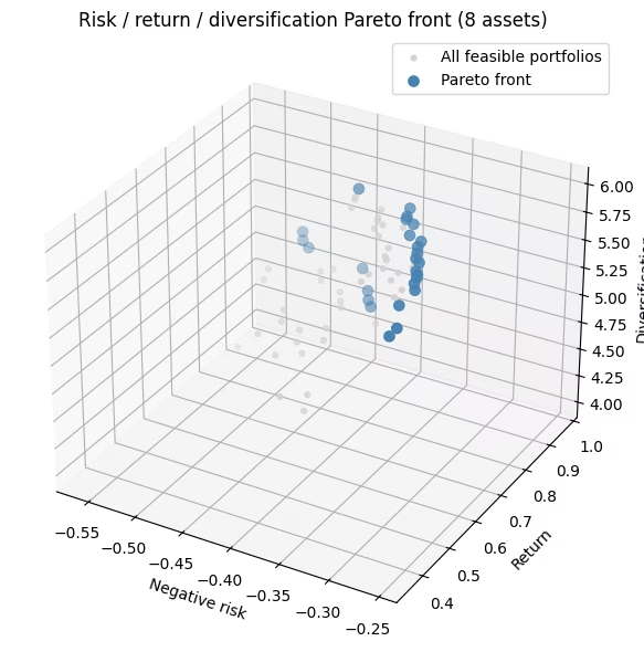
실현 가능한 포트폴리오(사후 선택 단계에서 얻은 정확히 $K$개의 자산)만 남기고, 각각을 세 가지 목표 모두에 대해 점수화한 뒤 파레토 프런티어를 추출합니다. 이는 모든 목표에서 동시에 다른 포트폴리오에 밀리지 않는 포트폴리오들입니다. 하이퍼볼륨은 프런티어가 지배하는 목적 공간의 크기를 요약한 하나의 숫자이며, 클수록 좋습니다.

256개의 비트열에 대해 100,000 샷을 실행하면 이 실행은 70개의 유효한 포트폴리오를 모두 보게 됩니다. 따라서 이 규모에서는 QAOA가 프런티어를 찾았다는 증거라기보다는, 파이프라인이 올바르게 연결되었는지 확인하는 사실상의 브루트 포스 검사입니다.

def evaluate_portfolio(bitstring, sigma, mu, D):
    """Score one portfolio on all three objectives (all framed as 'bigger is better')."""
    x = np.array([int(b) for b in bitstring])
    # negative risk, return, diversification (cross-sector pairs)
    return np.array([-(x @ sigma @ x), x @ mu, x @ D @ x])

# Post-select feasible portfolios, then score them.
feasible = [bs for bs in all_bitstrings if bs.count("1") == K]
fis = np.array([evaluate_portfolio(bs, sigma, mu, D) for bs in feasible])

pareto_front = filter_dominated(fis, maximise=True)
ref_point = fis.min(axis=0)
qmoo_hv = hypervolume(fis, ref=ref_point, maximise=True)

print(
    f"Feasible portfolios found : {len(feasible)} of {comb(n_assets, K)} possible"
)
print(f"Pareto-front portfolios   : {len(pareto_front)}")
print(f"Hypervolume               : {qmoo_hv:.4f}")

Feasible portfolios found : 70 of 70 possible
Pareto-front portfolios   : 26
Hypervolume               : 0.2487

fig = plt.figure(figsize=(8, 6))
ax = fig.add_subplot(111, projection="3d")
ax.scatter(
    fis[:, 0],
    fis[:, 1],
    fis[:, 2],
    c="lightgray",
    s=12,
    label="All feasible portfolios",
)
ax.scatter(
    pareto_front[:, 0],
    pareto_front[:, 1],
    pareto_front[:, 2],
    c="steelblue",
    s=45,
    label="Pareto front",
)
ax.set_xlabel("Negative risk")
ax.set_ylabel("Return")
ax.set_zlabel("Diversification")
ax.set_title("Risk / return / diversification Pareto front (8 assets)")
ax.legend()
plt.tight_layout()
plt.show()

대규모 하드웨어 예제

이제 40개 자산(8개 섹터 × 5)에서 $K=6$을 선택하는 동일한 워크플로를 실행합니다. 40개의 큐비트는 정확히 시뮬레이션하기에는 너무 크고($2^{40}$개의 진폭을 가진 상태벡터), 따라서 8개 자산일 때처럼 각도를 최적화할 수 없으며, 조밀한 회로는 현재 하드웨어에 비해 너무 깊습니다. $\binom{40}{6} \approx 3.8$M개의 유효한 포트폴리오는 고전적으로 열거할 수 있을 만큼 여전히 적어서, 마지막에 정확한 벤치마크로 사용합니다. 몇 가지가 달라지지만 방법 자체는 전혀 달라지지 않습니다.

1. 정확한 상태벡터가 아니라 행렬곱상태(MPS) 시뮬레이터로 각도를 학습합니다. 참고 문헌(Kotil 등)에 따라 목적 가중치를 동일한 값으로 고정하고, MPS 시뮬레이터에서 단일 β, γ를 최적화한 뒤 훑는 과정의 모든 가중치 벡터에 재사용합니다. (실행하는 크기에서 직접 학습하며, 작은 규모에서 큰 규모로 각도를 옮기지 않습니다.)

2. 하드웨어에 맞도록 위험 모델을 희소화합니다. 전체 공분산은 780개의 모든 자산 쌍을 결합합니다. 중요도 기반 QAP 절단을 사용해 가장 강하면서 라우팅 비용이 가장 낮은 결합만 남기고, 분산 항을 위해 각 섹터를 가벼운 고리로 결합합니다. 이렇게 하면 목적이 의미를 유지하면서도 회로를 하드웨어 친화적인 크기로 유지할 수 있습니다.

3. 회로를 얕게 유지하고 점수는 정직하게 매깁니다. 라우팅은 확률적이므로 여러 시드로 Transpile하여 가장 얕은 것을 유지합니다(양자 시간은 소비되지 않습니다). 포트폴리오는 항상 실제의 전체 목적에 대해 점수화됩니다. 희소화는 회로의 형태만 결정할 뿐 포트폴리오를 평가하는 방식에는 영향을 주지 않습니다.

QAP 절단을 쓰는 이유

각 자산에서 크기만 기준으로 가장 큰 결합을 남기면 희소하지만 라우팅하기는 여전히 까다로운 회로가 될 수 있습니다. 대신 QAP 절단은 크기가 크면서 동시에 칩에서 물리적으로 가까운 결합을 남기므로, 같은 게이트 예산으로 더 얕고 하드웨어 친화적인 회로를 얻을 수 있습니다.

1단계: 입력 매핑(하드웨어를 위해 희소화)

import csv
import urllib.request

# Download the committed market-data snapshot from the repo.
# --- 40-asset universe: 8 GICS sectors x 5 tickers (real market data) ---
# Load the committed market-data snapshot (real annualized returns and covariance).
# Values are stored at the precision used to train the shipped QAOA angles
# (mu: 3 dp, sigma: 4 dp), so the pre-trained parameters in instances/ stay exactly valid.

url = "https://raw.githubusercontent.com/Qiskit/documentation/main/datasets/tutorials/qmoo/market_data.csv"
urllib.request.urlretrieve(url, "market_data.csv")

with open("market_data.csv", newline="") as _f:
    _rows = list(csv.reader(_f))

# Covariance column order
_tickers_csv = _rows[0][2:]
# Asset tickers
tickers_40 = [r[0] for r in _rows[1:]]
# Annualized expected returns
mu_40 = np.array([float(r[1]) for r in _rows[1:]])
# Covariance (risk model)
sigma_40 = np.array([[float(v) for v in r[2:]] for r in _rows[1:]])

sectors_40 = [
    "Tech",
    "Tech",
    "Tech",
    "Tech",
    "Tech",
    "Energy",
    "Energy",
    "Energy",
    "Energy",
    "Energy",
    "Finance",
    "Finance",
    "Finance",
    "Finance",
    "Finance",
    "Health",
    "Health",
    "Health",
    "Health",
    "Health",
    "Staples",
    "Staples",
    "Staples",
    "Staples",
    "Staples",
    "Industrials",
    "Industrials",
    "Industrials",
    "Industrials",
    "Industrials",
    "Utilities",
    "Utilities",
    "Utilities",
    "Utilities",
    "Utilities",
    "REIT",
    "REIT",
    "REIT",
    "REIT",
    "REIT",
]
n_assets_40 = len(tickers_40)
K_40 = 6  # choose exactly K assets

sector_names_40 = list(dict.fromkeys(sectors_40))
sect_idx_40 = np.array([sector_names_40.index(s) for s in sectors_40])
# True cross-sector diversification matrix (used for scoring)
D_40 = np.array(
    [
        [
            0.5 if sectors_40[i] != sectors_40[j] else 0.0
            for j in range(n_assets_40)
        ]
        for i in range(n_assets_40)
    ]
)
np.fill_diagonal(D_40, 0.0)
print(
    f"{n_assets_40} assets, {len(sector_names_40)} sectors, choose K={K_40}"
)

40 assets, 8 sectors, choose K=6

# Sparsify the covariance so the risk circuit fits on hardware. A small diagonal
# shift (added after truncation) keeps the risk model positive semidefinite; at fixed
# K it adds the same constant to every portfolio, so it never changes the ranking.
# Importance-aware QAP truncation (Kotil et al. style): place the qubits on a line
# and use a Quadratic Assignment Problem to choose the layout that keeps the
# strongest covariance couplings within routing distance k of the swap network,
# then drop the rest. Unlike a fixed top-k cap, it keeps couplings that are both
# large AND cheap to route.
from scipy.optimize import quadratic_assignment as qap
from qiskit.transpiler.passes.routing.commuting_2q_gate_routing import (
    SwapStrategy,
)

# Truncation level: larger k keeps more couplings (deeper circuit)
k_truncate = 2
_dist = np.array(
    SwapStrategy.from_line(list(range(n_assets_40))).distance_matrix
)

def qap_truncate(Q, k):
    w = np.abs(Q.copy())
    np.fill_diagonal(w, 0.0)
    mask = (_dist <= k).astype(float)
    # Seed the QAP solver explicitly (by default it draws from NumPy's global
    # RNG, which SciPy is deprecating) so the truncation is reproducible.
    perm = qap(-w, mask, options={"rng": np.random.default_rng(42)}).col_ind
    keep = mask[np.ix_(perm, perm)]
    Qt = Q * keep
    np.fill_diagonal(Qt, np.diag(Q))
    return Qt

sigma_sparse = qap_truncate(sigma_40, k_truncate)
print(
    f"QAP truncation (k={k_truncate}): risk edges kept = "
    f"{(np.count_nonzero(sigma_sparse) - n_assets_40) // 2}"
)
ridge = max(0.0, -np.linalg.eigvalsh(sigma_sparse)[0]) + 1e-6
sigma_sparse = sigma_sparse + ridge * np.eye(n_assets_40)

# Diversity: couple each sector's assets in a ring (sparse stand-in for the
# same-sector pair count). Scoring still uses the true cross-sector matrix D_40.
def build_same_sector_hamiltonian(D_same, n):
    prob = OptimizationProblem("diversity_sparse")
    prob.binary_var_list(n)
    prob.minimize(quadratic=D_same)
    op, _ = prob.to_ising()
    return op.simplify()

D_ring = np.zeros((n_assets_40, n_assets_40))
for s in set(sect_idx_40):
    members = np.where(sect_idx_40 == s)[0]
    for k in range(len(members)):
        i, j = members[k], members[(k + 1) % len(members)]
        D_ring[i, j] = D_ring[j, i] = 0.5

H_risk_40 = build_risk_hamiltonian(sigma_sparse, n_assets_40)
H_return_40 = build_return_hamiltonian(mu_40, n_assets_40)
H_diversity_40 = build_same_sector_hamiltonian(D_ring, n_assets_40)
cost_ops_40 = [H_risk_40, H_return_40, H_diversity_40]
n_zz = sum(
    1 for p in sum(cost_ops_40).simplify().paulis if str(p).count("Z") == 2
)
print(
    f"Cost-layer interactions: {n_zz} (dense would be {n_assets_40*(n_assets_40-1)//2})"
)

QAP truncation (k=2): risk edges kept = 78
Cost-layer interactions: 102 (dense would be 780)

2-3단계: 각도를 학습한 다음 하드웨어 잡을 구성하고 제출

40개의 큐비트는 각도를 정확히 최적화하기에는 너무 크므로, 동일한 목적 가중치에서 행렬곱상태 시뮬레이터로 하나의 $\beta, \gamma$를 학습하고 훑는 과정 전체에서 재사용합니다. 아래 셀은 파일에서 미리 학습된 값을 불러옵니다. 학습된 비용 레이어 각도는 작아서 ($\gamma \approx 0.32$), 회로는 날카로운 사영이 아니라 완만한 편향을 적용합니다.

import json
from qiskit_ibm_runtime import QiskitRuntimeService, SamplerV2

# Pre-trained angles loaded from a file (training is slow; QDC pattern).
# Set load_params_file = False to retrain in-notebook.
load_params_file = True
params_url = "https://raw.githubusercontent.com/Qiskit/documentation/main/datasets/tutorials/qmoo/qaoa_params.json"
params_path = "qaoa_params.json"
if load_params_file:
    urllib.request.urlretrieve(params_url, params_path)
    qaoa_params = json.load(open(params_path))
    p_layers_hw = qaoa_params["p_layers"]
    opt_betas_40, opt_gammas_40 = qaoa_params["betas"], qaoa_params["gammas"]
else:
    # Same workflow as the small-scale example: qaoa_training_pipeline's MPSAerEvaluator
    # evaluates the QAOA energy on Aer's MPS simulator and supports the XY mixer.
    # As in the small-scale example the trainer maximizes energy, so we negate the
    # (to-be-minimized) objective sum; the 1/n_obj scaling matches the equal-weight
    # point of the sweep, so the trained gamma transfers directly to the weighted circuits.
    p_layers_hw = 1
    training_op_40 = sum(-1.0 / n_obj * H_k for H_k in cost_ops_40).simplify()

    dt = 0.75
    grid = np.arange(1, p_layers_hw + 1) - 0.5
    init_params_40 = np.concatenate(
        (1 - grid * dt / p_layers_hw, grid * dt / p_layers_hw)
    )

    trainer_40 = ScipyTrainer(
        MPSAerEvaluator({"matrix_product_state_max_bond_dimension": 24}),
        minimize_args={"options": {"maxiter": 80}},
    )
    print("Training QAOA angles (MPS simulator)...")
    result_train_40 = trainer_40.train(
        cost_op=training_op_40,
        mixer=xy_mixer(n_assets_40),
        initial_state=product_init(n_assets_40, K_40),
        params0=init_params_40,
    )
    opt_40 = result_train_40["optimized_params"]
    opt_betas_40, opt_gammas_40 = (
        list(opt_40[:p_layers_hw]),
        list(opt_40[p_layers_hw:]),
    )
    import os

    os.makedirs(os.path.dirname(params_path) or ".", exist_ok=True)
    json.dump(
        {
            "p_layers": p_layers_hw,
            "betas": opt_betas_40,
            "gammas": opt_gammas_40,
        },
        open(params_path, "w"),
        indent=2,
    )
    print(
        f"Trained angles saved to {params_path} (set load_params_file=True to reuse)."
    )

c40 = ParameterVector("c", n_obj)
# Negated to match the trained angles' sign, as in the small-scale cell; binding keeps +gamma.
combined_cost_op_40 = sum(
    -c40[k] * H_k for k, H_k in enumerate(cost_ops_40)
).simplify()
qc_40 = qaoa_ansatz(
    combined_cost_op_40,
    reps=p_layers_hw,
    initial_state=product_init(n_assets_40, K_40),
    mixer_operator=xy_mixer(n_assets_40),
)
qc_40.measure_all()
b40 = [p for p in qc_40.parameters if p.name.startswith("β")]
g40 = [p for p in qc_40.parameters if p.name.startswith("γ")]
pmap = {b40[i]: opt_betas_40[i] for i in range(p_layers_hw)}
pmap.update({g40[i]: opt_gammas_40[i] for i in range(p_layers_hw)})
ansatz_qc_40 = qc_40.assign_parameters(pmap)

service = QiskitRuntimeService()

# only use Heron devices
backend = service.least_busy(min_num_qubits=156)

# SABRE routing is stochastic: different seeds give different depths. Transpilation
# is classical (it costs no QPU time), so we transpile many seeds and keep only the
# shallowest circuit -- a free reduction in two-qubit depth before anything is sent
# to hardware. Only this single best circuit is ever executed.
n_seeds = 24
best = None
depths = []
for seed in range(n_seeds):
    pm = generate_preset_pass_manager(
        optimization_level=3, backend=backend, seed_transpiler=seed
    )
    qc = pm.run(ansatz_qc_40)
    d2 = qc.depth(lambda x: len(x.qubits) > 1)
    depths.append(d2)
    if best is None or d2 < best[0]:
        best = (d2, seed, qc)
isa_qc = best[2]
sd = sorted(depths)
print(
    f"Backend: {backend.name} | {n_seeds} seeds | two-qubit depth "
    f"best/median/worst = {sd[0]}/{sd[len(sd)//2]}/{sd[-1]} (best seed {best[1]})"
)
print(
    f"Selected circuit -> two-qubit gates: {isa_qc.num_nonlocal_gates()}, "
    f"two-qubit depth: {isa_qc.depth(lambda x: len(x.qubits) > 1)}"
)

Backend: ibm_kingston | 24 seeds | two-qubit depth best/median/worst = 220/261/300 (best seed 22)
Selected circuit -> two-qubit gates: 787, two-qubit depth: 220

# Submit one batched job (job mode; a single batch needs no Session).
# Extra shots: noise lowers the post-selection yield
n_samples_40, shots_40 = 24, 1500
c_vecs_40 = random_uniform_simplex(n_samples_40, n_obj)
sampler_hw = SamplerV2(mode=backend)
# Tag hardware jobs for tracking
sampler_hw.options.environment.job_tags = ["TUT_QAMOO"]
# Seconds; guard against runaway jobs
sampler_hw.options.max_execution_time = 600

# The QAOA angles are already bound; only the objective weights c remain free.
# Assign each weight vector to get one concrete circuit per point on the simplex.
bound_circuits_40 = [
    isa_qc.assign_parameters({c40[k]: cv[k] for k in range(n_obj)})
    for cv in c_vecs_40
]
job_hw = sampler_hw.run([(qc,) for qc in bound_circuits_40], shots=shots_40)
print(
    f"Submitted to {backend.name}: job id {job_hw.job_id()} ({len(bound_circuits_40)} circuits)"
)

Submitted to ibm_kingston: job id darcaalvr3kc73einokg (24 circuits)

4단계: 파레토 프런티어로 후처리하고 최적 포트폴리오 읽어내기

result_hw = job_hw.result()

# Post-select feasible portfolios (exactly K assets), score on the TRUE objectives.
feasible_40 = set()
for s in range(n_samples_40):
    for bs in result_hw[s].data.meas.get_counts():
        # get_counts is little-endian; reverse so bit i = asset i
        bs = bs.replace(" ", "")[::-1]
        if bs.count("1") == K_40:
            feasible_40.add(bs)

def score_40(P):
    """Score portfolios given as an (n, K) array of asset indices.

    Returns an (n, 3) array of [negative risk, return, diversification], all framed
    as 'bigger is better'. This is the single definition of the true objectives,
    used for the hardware samples, the exact enumeration, and the random baseline.
    Looping over the K x K index pairs keeps memory O(n) even for millions of rows.
    """
    risk = np.zeros(len(P))
    div = np.zeros(len(P))
    for a in range(P.shape[1]):
        for b in range(P.shape[1]):
            risk += sigma_40[P[:, a], P[:, b]]
            div += D_40[P[:, a], P[:, b]]
    return np.column_stack([-risk, mu_40[P].sum(1), div])

def evaluate_40(bs):
    """Score one bitstring (bit i = asset i) with score_40."""
    idx = np.flatnonzero([b == "1" for b in bs])
    return score_40(idx[None, :])[0]

fis_40 = np.array([evaluate_40(bs) for bs in feasible_40])
pareto_40 = filter_dominated(fis_40, maximise=True)
print(f"Feasible portfolios collected : {len(feasible_40)}")
print(f"Pareto-front portfolios       : {len(pareto_40)}")

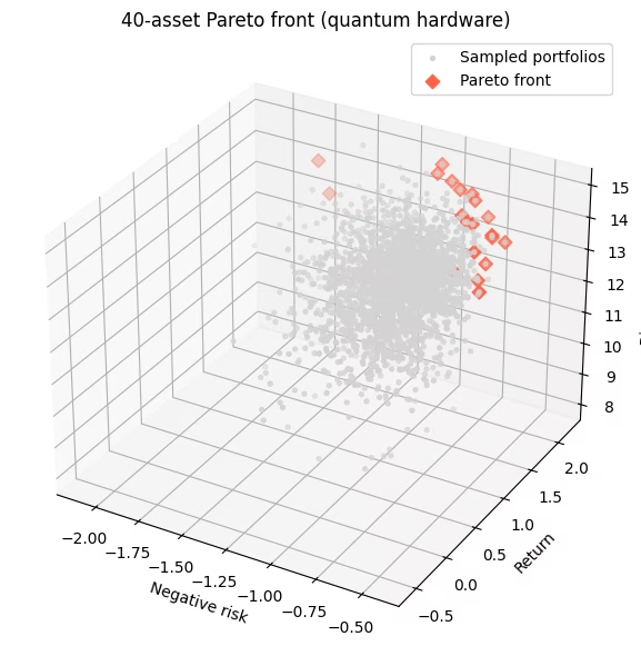
Feasible portfolios collected : 2359
Pareto-front portfolios       : 20

# --- Honest benchmark: QAOA and random vs the EXACT Pareto front ---
# 40 choose 6 = 3,838,380 feasible portfolios -- few enough to enumerate exactly, score
# every one on the TRUE objectives, and get the exact Pareto front. That front is an
# absolute ceiling, and its feasible nadir is a FIXED hypervolume reference point, so the
# numbers are comparable across runs instead of depending on what happened to be sampled.
import itertools

# Stream the combinations straight into an (n, K) index array, without first
# building millions of Python tuples.
combos = np.fromiter(
    itertools.chain.from_iterable(
        itertools.combinations(range(n_assets_40), K_40)
    ),
    dtype=np.int16,
).reshape(-1, K_40)
fis_exact = score_40(combos)
front_exact = filter_dominated(fis_exact, maximise=True)

# Fixed reference = worst value of each objective over ALL feasible portfolios (the nadir).
ref_fixed = fis_exact.min(axis=0)
# The hypervolume of a point set equals the hypervolume of its front.
hv_ceiling = hypervolume(front_exact, ref=ref_fixed, maximise=True)
hv_qaoa = hypervolume(fis_40, ref=ref_fixed, maximise=True)

def random_feasible_hv(n_draw, seed):
    """Hypervolume of n_draw uniformly-random feasible portfolios, same fixed reference."""
    rng = np.random.default_rng(seed)
    picks = set()
    while len(picks) < n_draw:
        picks.add(tuple(sorted(rng.choice(n_assets_40, K_40, replace=False))))
    P = np.array(list(picks))
    return hypervolume(score_40(P), ref=ref_fixed, maximise=True)

hv_rand = np.array(
    [random_feasible_hv(len(feasible_40), seed) for seed in range(20)]
)

print(f"Exact Pareto front            : {len(front_exact)} portfolios")
print(f"Hypervolume ceiling (optimum) : {hv_ceiling:.3f}")
print(
    f"QAOA (hardware)               : {100 * hv_qaoa / hv_ceiling:5.1f}% of optimum"
)
print(
    f"Random ({len(feasible_40)} draws, 20 seeds) : "
    f"{100 * hv_rand.mean() / hv_ceiling:5.1f}% +/- {100 * hv_rand.std() / hv_ceiling:.1f}% of optimum"
)

Exact Pareto front            : 61 portfolios
Hypervolume ceiling (optimum) : 64.211
QAOA (hardware)               :  85.5% of optimum
Random (2359 draws, 20 seeds) :  84.4% +/- 1.3% of optimum

이 문제 크기에서 QAOA는 균등 무작위 샘플링과 거의 비슷한 성능을 보입니다. 둘 다 정확한 최적해 하이퍼볼륨의 상당 부분을 복원하며, 어느 쪽도 뚜렷하게 앞서지 않습니다. 이 결과는 잡음이 있는 하드웨어에서 크게 절단된 비용 연산자를 가진 단일 얕은 QAOA 레이어에서는 예상되는 것입니다. 이 예제의 가치는 양자 속도 향상이 아니라 종단 간 다목적 워크플로(매핑, 각도 학습, 제약 샘플링, 파레토 후처리)에 있습니다. 최적해와의 격차를 줄이려면 더 깊은 회로(더 많은 QAOA 레이어), 더 완만한 절단, 또는 더 낮은 잡음의 하드웨어가 필요합니다.

# The best trade-offs found by the sampler: no other sampled portfolio beats these
# on every objective. They approximate the exact front computed above; a
# decision-maker picks the trade-off they prefer.
bs_list = list(feasible_40)
# Boolean mask over fis_40; keep_weakly=True also keeps portfolios whose
# objective values tie with a front point (what the strict filter would drop).
mask = is_nondominated(fis_40, maximise=True, keep_weakly=True)
front_bs = [b for b, m in zip(bs_list, mask) if m]
front_f = fis_40[mask]
order = np.argsort(-front_f[:, 1])  # show a span sorted by return
print(
    f"{mask.sum()} non-dominated sampled portfolios. A representative span:\n"
)
print(
    f"{'tickers held':40s} {'risk':>7s} {'return':>7s} {'cross-sector':>12s}"
)
for idx in order[:: max(1, len(order) // 12)]:
    held = [tickers_40[i] for i, b in enumerate(front_bs[idx]) if b == "1"]
    print(
        f"{', '.join(held):40s} {-front_f[idx,0]:7.3f} {front_f[idx,1]:7.2f} {int(front_f[idx,2]):12d}"
    )

fig = plt.figure(figsize=(8, 6))
ax = fig.add_subplot(111, projection="3d")
ax.scatter(
    fis_40[:, 0],
    fis_40[:, 1],
    fis_40[:, 2],
    c="lightgray",
    s=8,
    label="Sampled portfolios",
)
ax.scatter(
    pareto_40[:, 0],
    pareto_40[:, 1],
    pareto_40[:, 2],
    c="tomato",
    marker="D",
    s=40,
    label="Pareto front",
)
ax.set_xlabel("Negative risk")
ax.set_ylabel("Return")
ax.set_zlabel("Diversification")
ax.set_title("40-asset Pareto front (quantum hardware)")
ax.legend()
plt.tight_layout()
plt.show()

20 non-dominated sampled portfolios. A representative span:

tickers held                                risk  return cross-sector
AAPL, NVDA, XOM, GS, BLK, CAT              1.715    2.22           13
NVDA, GS, MS, PFE, CAT, PLD                1.772    2.20           14
NVDA, MS, PFE, WMT, CAT, DUK               1.040    2.14           15
NVDA, CVX, GS, JNJ, KO, WMT                0.737    2.01           14
NVDA, COP, GS, JNJ, WMT, EQIX              1.014    1.98           15
NVDA, ABT, WMT, CAT, AEP, EQIX             0.913    1.92           15
NVDA, CVX, WMT, RTX, D, EQIX               0.835    1.82           15
NVDA, XOM, GS, JNJ, DUK, EQIX              0.763    1.80           15
AAPL, NVDA, JNJ, KO, RTX, SO               0.621    1.71           14
NVDA, CVX, BLK, JNJ, RTX, AEP              0.719    1.71           15
NVDA, JNJ, KO, COST, RTX, AEP              0.545    1.69           14
NVDA, CVX, ABT, WMT, HON, AEP              0.702    1.43           15
AAPL, GS, JNJ, PEP, AEP, EQIX              0.645    1.34           15
MSFT, XOM, BLK, JNJ, CAT, SO               0.617    1.34           15
MSFT, KO, WMT, RTX, SO, SPG                0.526    1.29           14
MSFT, XOM, BLK, JNJ, WMT, DUK              0.483    1.25           15
MSFT, CVX, JNJ, RTX, DUK, D                0.482    1.02           14
MSFT, XOM, JNJ, KO, HON, EQIX              0.479    0.93           15
MSFT, JNJ, PG, KO, RTX, DUK                0.423    0.86           14
MSFT, XOM, JNJ, PEP, DUK, AMT              0.476    0.57           15

다음 단계

추천 자료

이 튜토리얼이 흥미로웠다면 다음을 고려해 보세요.

• 다운로드한 시장 데이터(market_data.csv)를 실제 가격 이력에서 얻은 자신의 수익률 및 공분산 추정치로 바꿔 보세요.

• QAOA 레이어 수를 늘리거나, 12–16개 자산에서 학습한 각도를 옮겨 와서 하드웨어 프런티어를 최적에 더 가깝게 만들어 보세요.

• Kotil 등의 Quantum Approximate Multi-Objective Optimization (Nature Computational Science, 2025)을 읽어 보세요. 이 튜토리얼이 포트폴리오에 맞게 적용한 맥스컷 연구입니다.

참고 문헌

1. Kotil et al., "Quantum Approximate Multi-Objective Optimization," Nature Computational Science (2025). arXiv:2503.22797

2. S. H. Sack and M. Serbyn, "Quantum annealing initialization of the quantum approximate optimization algorithm," Quantum 5, 491 (2021). arXiv:2101.05742