클래시컬 섀도로 잡음이 있는 양자 상태 학습하기
사용량 추정: Heron r2 프로세서에서 34분 (참고: 추정치일 뿐이며 실제 실행 시간은 다를 수 있습니다.)
학습 목표
-
Julia에서 IBM® 양자 프로세서의 무작위 측정을 수집하고 나중에 분석할 수 있도록 저장합니다
-
학습 전에 측정 데이터에서 결함이 있는 큐비트와 게이트를 확인합니다
-
노이즈가 있는 상태의 행렬 곱 연산자(MPO) 모델을 classical shadow에 맞춰 피팅합니다
-
보류한(held-out) 측정으로 모델을 검증하고 이상적인 회로와 비교합니다
사전 지식
-
Greenberger-Horne-Zeilinger(GHZ) 상태의 Shadow tomography 튜토리얼에서 소개한 classical shadow
-
양자 정보의 기초에서 다루는 밀도 행렬과 혼합 상태
-
횡자기장 Ising 모델의 시간 발전 시뮬레이션 튜토리얼에서 소개한
Qiskit.jl과QiskitIBMRuntime.jl을 사용한 Julia에서의 회로 실행
배경
실제 양자 프로세서에서는 노이즈 때문에 회로가 준비하도록 설계된 순수 상태 가 혼합 상태 로 바뀝니다. 전체 양자 상태 tomography로 를 재구성할 수 있지만, 필요한 측정 횟수는 큐비트 수에 따라 지수적으로 증가합니다. 대신 Votto 등 [1]은 무작위 측정으로부터 최대 96큐비트까지의 에 대한 간결한 모델을 학습했습니다. 이 튜토리얼은 그들의 워크플로를 따릅니다.
무작위 측정 [2]에서는 모든 큐비트 를 독립적인 무작위 유니터리 로 회전한 다음 계산 기저에서 측정합니다. 회전을 한 번 뽑은 것을 측정 설정(measurement setting)이라고 하며, 각 설정은 shot 동안 반복됩니다. 결과 비트가 인 shot 하나는 classical shadow [3]를 줍니다.
이 shadow를 설정과 shot에 대해 평균하면 가 됩니다. 사전 지식 튜토리얼에서는 각 를 세 가지 Pauli 기저에서 뽑지만, 이 튜토리얼은 논문과 마찬가지로 모든 단일 큐비트 유니터리에서 균일하게(Haar 무작위) 뽑으며, 같은 공식이 적용됩니다.
Shadow는 한 번에 소수의 큐비트에 대한 성질을 추정합니다. 논문은 이를 행렬 곱 연산자(MPO)로 결합합니다. MPO는 밀도 행렬을 큐비트당 하나씩 작은 텐서의 사슬로 나타내며, 단거리 상관관계를 갖는 노이즈 상태는 이웃한 텐서 사이에 작은 본드만 있으면 됩니다. 밀도 행렬 재규격화 군(DMRG) 알고리즘처럼 학습기는 사슬을 따라 sweep하면서 한 번에 텐서 하나를 갱신하여, 해당 텐서를 중심으로 하는 개 큐비트의 윈도우에서 모델이 shadow와 일치하도록 합니다(논문의 식 4). 이러한 갱신 동안 본드 차원은 고정되므로 학습기는 모델을 절단하지 않습니다. 데이터가 이 윈도우를 통해서만 들어오기 때문에, 필요한 설정 수는 사슬의 길이에 따라 증가하지 않습니다.
설정은 훈련 세트와 테스트 세트로 나뉩니다. 논문은 테스트 세트에서 와 모델 사이의 최대 충실도(max fidelity)를 추정합니다.
를 직접 측정하려면 지수적으로 많은 측정이 필요합니다. 대신 논문은 근사 인수분해 조건(AFC)을 가정합니다. 즉 의 상관관계가 몇 개의 큐비트 안에서 감쇠하므로, 전역 중첩과 순도는 이웃한 개 큐비트 블록에 대한 항으로 인수분해됩니다. 순도로부터 Rényi-2 엔트로피 도 얻을 수 있으며, 이는 상태가 얼마나 혼합되어 있는지를 나타냅니다.
논문은 깊이 의 kicked-Ising 상태를 준비합니다.
Eagle 프로세서인 ibm_brisbane의 96큐비트에서, 에 대해 1,024 shot씩 2,048개 설정으로 준비합니다. 논문의 그림 1(c,d)는 에 대한 두 가지 결과를 보고합니다.
-
학습된 모델은 에서 실험 상태와 에 도달하며, 이는 이상적인 상태 와 실험 상태의 중첩보다 훨씬 높습니다.
-
엔트로피는 으로 선형적으로 증가하며, 모델의 엔트로피는 테스트 세트에서 얻은 독립적인 추정값과 일치합니다.
이 튜토리얼은 두 결과를 모두 확인합니다. 먼저 정확한 답을 아는 8큐비트 시뮬레이션에서 확인하고, 그다음 Heron r2 프로세서인 ibm_fez에서 새로 실행한 96큐비트 실험에서 확인합니다. 학습기는 논문과 보충 자료의 방정식을 독립적으로 구현한 Julia 코드입니다.
요구 사항
Qiskit.jl이 아직 Windows를 지원하지 않으므로(Qiskit.jl issue #15) 이 튜토리얼에는 macOS 또는 Linux가 필요합니다. 또한 다음이 필요합니다.
-
Julia 다운로드 페이지 또는
juliaup add 1.11로 설치한 Julia 1.11, 그리고IJulia패키지:julia -e 'using Pkg; Pkg.add("IJulia")' -
하드웨어 예제에는 96큐비트 이상의 QPU에 접근할 수 있는 IBM Quantum® Platform 계정과 저장된 자격 증명이 필요합니다. 계정이 없다면, 이 튜토리얼의 결과를 만들어 낸
ibm_fez실행의 저장된 측정값으로 하드웨어 예제를 실행할 수 있습니다. 나머지 섹션은 계정 없이 실행됩니다.
이 노트북은 회로를 만들고 실행하기 위해 Qiskit.jl과 QiskitIBMRuntime.jl을, 무작위 측정을 위해 RandomMeas.jl [4]을(ITensors.jl과 ITensorMPS.jl도 함께 제공합니다), 그리고 NPZ.jl, JSON.jl, Plots.jl을 사용합니다. 이 튜토리얼은 Qiskit.jl 0.6.1, QiskitIBMRuntime.jl 0.3.2, RandomMeas.jl 0.3.1로 테스트되었습니다.
환경을 설정하는 방법은 두 가지입니다.
-
옵션 1: 호환되는 최신 버전의 패키지를 임시 환경에 설치합니다. 다음 셀을 수정하지 않고 실행하세요.
-
옵션 2: 테스트된 환경을 그대로 재현합니다. 다음 셀에서
download_toml_files = true로 설정하세요. 이 셀은 문서 저장소에서Project.toml과Manifest.toml을 이 노트북 옆의env_tutorial/classical-shadows/폴더로 내려받은 다음, 간접 의존성을 포함하여 manifest에 기록된 모든 패키지의 정확한 버전을 설치합니다. 자세한 내용은 이 파일들에 대한 Julia 문서를 참조하세요.
using Pkg
using Downloads

download_toml_files = false

if !download_toml_files
    # Option 1: Install the latest compatible versions into a temporary environment
    Pkg.activate(mktempdir(); io=devnull)
    Pkg.add([
        PackageSpec(name="Qiskit", version="0.6"),
        PackageSpec(name="QiskitIBMRuntime", version="0.3"),
        PackageSpec(name="RandomMeas", version="0.3"),
        PackageSpec(name="NPZ"),
        PackageSpec(name="JSON"),
        PackageSpec(name="Plots"),
    ]; io=devnull)
else
    # Option 2: Install the exact tested versions recorded in Project.toml and Manifest.toml
    base_url = "https://raw.githubusercontent.com/Qiskit/documentation/main/docs/tutorials/assets/classical-shadows/julia"
    env_dir = joinpath(@__DIR__, "env_tutorial", "classical-shadows")
    mkpath(env_dir)
    for file in ("Project.toml", "Manifest.toml")
        Downloads.download("$base_url/$file", joinpath(env_dir, file))
    end
    Pkg.activate(env_dir; io=devnull)
    Pkg.instantiate(; io=devnull)
end
설정
using RandomMeas  # also loads ITensors and ITensorMPS
using Qiskit, QiskitIBMRuntime
using Random, LinearAlgebra, Statistics
using Downloads, SHA, NPZ, JSON, Plots

# Download the helper module that implements the learner, unless a copy exists
docs_url = "https://raw.githubusercontent.com/Qiskit/documentation/main"
helper_file = joinpath(@__DIR__, "env_tutorial", "classical-shadows", "mpo_learning.jl")
if !isfile(helper_file)
    mkpath(dirname(helper_file))
    helper_url = "$docs_url/docs/tutorials/assets/classical-shadows/julia/mpo_learning.jl"
    Downloads.download(helper_url, helper_file)
end
include(helper_file)
using .ShadowMPOLearning
BLAS.set_num_threads(1)  # the learner multiplies many small matrices
Setup 셀이 내려받는 도우미 모듈 mpo_learning.jl이 학습기를 구현합니다. 이 튜토리얼은 여기서 다음 함수들을 호출합니다.
| 함수 | 용도 |
|---|---|
kicked_ising_reference(N, D; depolarization) | 이상적인 kicked-Ising 상태 또는 국소 탈분극 노이즈 이후 상태의 정확한 MPO |
split_settings(group; seed, train_fraction) | 측정 설정을 훈련 세트와 테스트 세트에 무작위로 배정(기본값은 각각 절반) |
training_marginals(train; ell, prior) | 훈련 설정만을 사용한, 모든 학습 윈도우의 shadow 추정값 |
fitted_prior(ideal, train) | 논문에서처럼 각 윈도우의 측정된 순도에 맞춰 피팅한, 공통 무작위 측정(CRM)의 사전 분포 |
learn_mpo(marginals, N; ell, maxbond, sweeps) | 최대 혼합 상태에서 시작하여 논문의 단일 사이트 갱신을 사슬을 따라 sweep |
max_fidelity(a, b), mpo_overlap(a, b) | 두 MPO 사이의 정확한 와 |
afc_estimate, afc_statistics, afc_prefix_curve | jackknife 오차 막대를 갖는, 테스트 설정으로부터의 와 의 AFC 추정값 |
학습기는 MPO를 Pauli 기저로 저장합니다. 이렇게 하면 모델이 에르미트이고 대각합이 1로 유지되지만, 모델이 양의 반정부호가 되도록 강제하지는 않습니다. 따라서 노트북은 고유값이 얼마나 음수가 되는지 보고합니다.
소규모 시뮬레이터 예제
모든 것을 정확하게 계산할 수 있을 만큼 작은 시스템, 즉 8큐비트의 깊이 1 kicked-Ising 상태에서 시작합니다. 하드웨어를 모사하기 위해 12%의 국소 탈분극 노이즈를 적용합니다. 노이즈가 있는 상태를 알고 있으므로 학습된 모델을 그것과 직접 비교할 수 있습니다.
1단계: 고전 입력을 양자 문제로 매핑
kicked_ising_reference 함수는 정확한 상태를 MPO로 반환합니다. depolarization=0.12이면 회로 이후 모든 큐비트의 Bloch 벡터가 12% 줄어듭니다.
N = 8
ideal = kicked_ising_reference(N, 1)
rho = kicked_ising_reference(N, 1; depolarization=0.12)
println("Purity of the noisy state: ", round(mpo_overlap(rho, rho), digits=3))
println("F_max between the noisy and ideal states: ", round(max_fidelity(rho, ideal), digits=3))
Purity of the noisy state: 0.327
F_max between the noisy and ideal states: 0.56
2단계: 양자 하드웨어 실행에 맞게 문제 최적화
이 예제는 측정 결과를 고전적으로 샘플링하므로 트랜스파일할 회로가 없습니다. 이 단계는 하드웨어 예제에서 다룹니다.
3단계: Qiskit primitive를 사용하여 실행
RandomMeas.jl을 사용하여 Haar 무작위 측정 설정 2,048개를 뽑고 각각에서 256 shot을 샘플링한 다음, 설정을 훈련 세트와 테스트 세트로 균등하게 나눕니다. shot이 아니라 설정 단위로 나누세요. 같은 설정의 shot은 그 설정의 회전을 공유하므로 서로 독립적이지 않습니다.
Random.seed!(20260921)
sites = siteinds("Qubit", N)
settings = [LocalUnitaryMeasurementSetting(N; site_indices=sites, ensemble=Haar) for _ in 1:2048]
measurements = MeasurementGroup(to_itensor_mpo(rho, sites), settings, 256)
split = split_settings(measurements; seed=20260921)
println(length(split.train_ids), " training settings, ", length(split.test_ids), " testing settings")
1024 training settings,
1024 testing settings
4단계: 후처리하여 원하는 고전 형식으로 결과 반환
논문의 깊이 1 매개변수로 모델을 학습합니다. 갱신하는 텐서의 양쪽으로 개 큐비트씩 확장되는 윈도우, 본드 차원 4, 최대 혼합 상태에서 시작하는 20회 sweep을 사용합니다. 첫 번째 sweep은 이웃한 텐서 쌍을 갱신하여 본드 차원이 1에서 4까지 늘어나게 하고, 이후의 모든 sweep은 그 고정된 본드 차원에서 한 번에 텐서 하나를 갱신합니다.
shadow의 통계적 노이즈를 줄이기 위해 논문은 공통 무작위 측정(CRM) [5]을 사용합니다. 각 설정에 대해, 상태에 대한 사전 추정이 같은 설정에서 만들어 낼 평균 shadow를 빼고, 그런 다음 사전 분포의 정확한 값을 다시 더합니다. 이 보정은 평균이 0이므로, 사전 분포는 통계 오차의 크기만 바꿀 뿐 추정 대상은 바꾸지 않습니다. 여기서 사전 분포는 10% 국소 탈분극이 있는 이상적인 상태로, 실제 값 12%에 가깝습니다. 하드웨어에서는 노이즈 수준을 알 수 없으므로, 하드웨어 예제는 논문처럼 사전 분포를 측정된 순도에 맞춰 피팅합니다.
prior = kicked_ising_reference(N, 1; depolarization=0.10)
marginals = training_marginals(split.train; ell=2, prior)
fit = learn_mpo(marginals, N; ell=2, maxbond=4, sweeps=20)
sigma = fit.model
plot([h.sweep for h in fit.history], [h.local_loss for h in fit.history];
    xlabel="sweep", ylabel="mean squared residual", label="training windows",
    size=(680, 320), left_margin=5Plots.mm, bottom_margin=5Plots.mm)
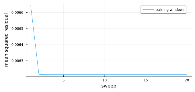
잔차는 모델의 윈도우가 훈련 shadow에서 얼마나 떨어져 있는지를 나타냅니다. 단일 사이트 갱신이 시작되는 두 번째 sweep에서 감소한 뒤 0에 도달하지 않고 대략 일정하게 유지되는데, shadow에는 작은 본드 차원의 모델로는 재현할 수 없는 통계적 노이즈가 있기 때문입니다.
이 상태를 알고 있으므로 학습된 모델을 그것과 정확하게 비교할 수 있고, 가장 단순한 두 가지 추측인 CRM 사전 분포와 이상적인 상태도 함께 비교할 수 있습니다.
eigenvalues = eigvals(Hermitian(dense_operator(sigma)))
println("F_max with the noisy state")
println("  learned model: ", round(max_fidelity(rho, sigma), digits=3))
println("  CRM prior:     ", round(max_fidelity(rho, prior), digits=3))
println("  ideal state:   ", round(max_fidelity(rho, ideal), digits=3))
println("Most negative eigenvalue of the model: ", round(minimum(eigenvalues), digits=4))
println("Total negative eigenvalue weight:      ", round(-sum(min.(eigenvalues, 0)), digits=4))
F_max with the noisy state
learned model: 0.993
  CRM prior:     0.911
  ideal state:   0.56
Most negative eigenvalue of the model: -0.0076
Total negative eigenvalue weight:      0.0348
학습된 모델은 사전 분포나 이상적인 상태보다 노이즈가 있는 상태에 더 가까우므로, 데이터로부터 노이즈를 학습한 것입니다. 모델의 작은 음의 고유값은 유한한 측정 횟수에서 비롯됩니다.
하드웨어에서는 상태를 알 수 없으므로 대신 테스트 설정으로부터 를 추정합니다. AFC는 사슬을 개 큐비트로 이루어진 블록 로 나누고 순도를 다음과 같이 근사합니다.
그리고 는 국소 중첩의 같은 비율로 근사합니다. 이면 두 블록이 8개 큐비트를 모두 덮으므로 공식은 정확하고, 이면 인수분해 가정에 의존합니다. 테스트 설정을 한 번에 하나씩 제외하는 jackknife 오차 막대는 테스트 데이터의 통계 오차만 포함하며, 훈련의 무작위성이나 AFC 근사는 포함하지 않습니다.
for k in (2, 4)
    estimate = afc_estimate(sigma, split.test; k, statistics=afc_statistics(split.test, k; prior))
    println("k = $k: held-out F_max = ", round(estimate.fidelity, digits=3), " ± ",
        round(estimate.fidelity_sem, digits=3))
end
println("Exact F_max:              ", round(max_fidelity(rho, sigma), digits=3))
k = 2: held-out F_max = 0.966
± 0.036
k = 4: held-out F_max =
0.958 ± 0.049
Exact F_max:              0.993
보류한 두 추정값 모두 오차 막대 범위 안에서 정확한 값과 일치합니다.
대규모 하드웨어 예제
이제 Heron r2 프로세서인 ibm_fez의 96큐비트 사슬에서 실험을 실행합니다. ibm_brisbane처럼 heavy-hex 커플링 맵을 가지며 노이즈 수준도 비슷합니다.
데이터를 수집하려면 Sampler 작업 1,024개와 약 34분의 QPU 시간이 필요합니다. 96큐비트 이상의 QPU에 접근할 수 없거나 대기열이 길다면, 이 튜토리얼에 표시된 결과를 만들어 낸 2026년 9월 27일의 ibm_fez 측정값으로 하드웨어 예제를 실행하세요. use_saved_data = true이면 노트북이 1단계에서 Zenodo [6]로부터 이 측정값(15 MB)을 내려받고 3단계에서 작업 제출을 건너뜁니다. 직접 데이터를 수집하려면 false로 설정하세요.
use_saved_data = true; # set to false to collect new measurements on hardware
1단계: 고전 입력을 양자 문제로 매핑
각 설정에는 회로가 하나씩 필요합니다. kicked-Ising 회로, 를 위해 각 큐비트에 적용하는 gate, 그리고 모든 큐비트의 측정으로 구성됩니다. , , 가 에서 균일하도록 를 샘플링하면 가 Haar 무작위가 됩니다. u3_matrix 함수는 4단계에서 사용하는 의 행렬을 반환합니다.
예산은 1,024 shot씩 1,024개 설정으로, 논문의 설정 수의 절반이며 훈련과 테스트에 균등하게 나눕니다. 저장된 데이터를 사용하면 셀이 기록된 각도를 불러옵니다. 그렇지 않으면 새 각도를 뽑아 아무것도 제출하기 전에 저장하는데, 각도가 없으면 결과를 분석할 수 없기 때문입니다. 파일이 이미 있으면 셀이 이를 불러오므로, 세션을 다시 시작한 후에도 각도가 저장된 결과와 계속 일치합니다.
"Matrix of the U(θ, ϕ, λ) gate, as used by `qc.u` in Qiskit."
u3_matrix(θ, ϕ, λ) = [cos(θ/2)              -exp(im*λ)*sin(θ/2);
                      exp(im*ϕ)*sin(θ/2)    exp(im*(ϕ + λ))*cos(θ/2)]

"Angles (θ, ϕ, λ) for which `u3_matrix(θ, ϕ, λ)` is a Haar-random unitary."
random_u3_angles() = (2asin(sqrt(rand())), 2π*rand(), 2π*rand())

N_hw, NU_hw, NM_hw = 96, 1024, 1024
data_directory = joinpath(@__DIR__, "classical-shadows-data")
saved_file = joinpath(data_directory, "ibm-fez-run.npz")
run_directory = joinpath(data_directory, "new-run")
settings_file = joinpath(run_directory, "settings.npz")
if use_saved_data
    saved_url = "https://zenodo.org/records/24116174/files/ibm-fez-run.npz?download=1"
    saved_sha256 = "c42f4d8d42e5083e9e152b4fec0846884ebe3be003e5ab528deebf4f00c9fe50"
    if !isfile(saved_file)
        mkpath(data_directory)
        println("Downloading the saved ibm_fez run (15 MB)...")
        Downloads.download(saved_url, saved_file * ".part")
        mv(saved_file * ".part", saved_file)
    end
    bytes2hex(open(sha256, saved_file)) == saved_sha256 ||
        error("$saved_file is incomplete or corrupted; delete it and run this cell again")
    saved_run = npzread(saved_file)
    angles = saved_run["angles"]
elseif isfile(settings_file)
    angles = npzread(settings_file)["angles"]
else
    mkpath(joinpath(run_directory, "outcomes"))
    Random.seed!(20260927)
    angles = Array{Float64}(undef, NU_hw, N_hw, 3)
    for r in 1:NU_hw, i in 1:N_hw
        angles[r, i, :] .= random_u3_angles()
    end
    npzwrite(settings_file, Dict("angles" => angles))
end
println("Measurement settings: ", size(angles, 1), " × ", size(angles, 2), " qubits")
Measurement settings: 1024
× 96 qubits
2단계: 양자 하드웨어 실행에 맞게 문제 최적화
사슬은 가장 나쁜 큐비트만큼만 좋으므로, 96개의 물리 큐비트를 직접 선택하세요. Qiskit.jl의 transpile 함수는 아직 고정된 초기 레이아웃을 받을 수 없으며, ibm_phoenix에서의 테스트에서 이 함수가 선택한 레이아웃에는 판독 오류가 51%인 큐비트가 포함되어 있었습니다. 다음 사슬은 Python Qiskit transpile 함수(optimization_level=3)의 오류 인식 레이아웃이 2026년 9월 27일의 보정 데이터에서 선택한, ibm_fez 커플링 맵의 96큐비트 경로입니다. 평균 판독 오류는 1.6%이지만 heavy-hex 격자에는 96큐비트 경로가 많지 않고, 이 경로에는 판독 오류가 15%인 큐비트 35가 포함되어 있습니다. 보정은 바뀌므로, 다른 날이나 다른 QPU에서 실행하기 전에 현재의 보정 데이터에서 새 사슬을 선택하세요.
이 사슬을 유지하려면 회로를 트랜스파일하지 말고 네이티브 gate로 직접 작성하세요. gate는 전역 위상을 제외하면 와 같습니다. 이 분해는 무작위 회전과 킥 를 모두 포함합니다. gate 는 전역 위상을 제외하면 CZ gate 뒤에 두 큐비트 모두에 를 적용한 것과 같습니다. 이 gate는 대각이므로 CZ gate와 교환되고, 따라서 각 큐비트는 측정 회전 전에 본드마다 를 하나씩 모으게 됩니다.
num_device_qubits = 156
# Physical qubits of ibm_fez, in IBM numbering, forming the chain
chain_physical = [
    2, 3, 4, 5, 6, 7, 8, 9, 10, 11, 12, 13, 14, 15, 19, 35, 34, 33, 39, 53, 54, 55, 59, 75, 74,
    73, 79, 93, 94, 95, 99, 115, 114, 113, 119, 133, 132, 131, 130, 129, 128, 127, 137, 147, 146,
    145, 144, 143, 136, 123, 124, 125, 117, 105, 106, 107, 108, 109, 110, 111, 98, 91, 90, 89,
    88, 87, 86, 85, 77, 65, 66, 67, 68, 69, 70, 71, 58, 51, 50, 49, 48, 47, 46, 45, 37, 25, 24,
    23, 22, 21, 36, 41, 42, 43, 56, 63]
chain = chain_physical .+ 1  # Qiskit.jl numbers qubits from 1

"Apply U(θ, ϕ, λ) to qubit q with native gates: rz(λ), sx, rz(θ + π), sx, rz(ϕ + π)."
function native_u!(qc, q, θ, ϕ, λ)
    qc.rz(λ, q)
    qc.sx(q)
    qc.rz(θ + π, q)
    qc.sx(q)
    qc.rz(ϕ + π, q)
end

"Kicked-Ising circuit on `chain`, then the rotations of one setting and a measurement."
function native_setting_circuit(chain, angles, num_device_qubits)
    n = length(chain)
    qc = QuantumCircuit(num_device_qubits, n)
    for q in chain
        native_u!(qc, q, π/4, -π/2, π/2)       # e^{-iπ/8 X}
    end
    for i in 1:n-1
        qc.cz(chain[i], chain[i + 1])          # e^{iπ/4 ZZ}, up to the S† gates below
    end
    for (i, q) in enumerate(chain)
        bonds = (i > 1) + (i < n)
        qc.rz(-π/2 * bonds, q)                 # one S† per bond
        native_u!(qc, q, angles[i, 1], angles[i, 2], angles[i, 3])
        qc.measure(q, i)                       # outcome of chain qubit i goes to bit i
    end
    qc
end

circuits = [native_setting_circuit(chain, angles[r, :, :], num_device_qubits) for r in 1:NU_hw]
println(length(circuits), " circuits, each with ", count(inst -> inst.name == "cz", circuits[1].data), " CZ gates")
1024 circuits, each with
95 CZ gates
3단계: Qiskit primitive를 사용하여 실행
QiskitIBMRuntime.jl은 Sampler 작업 하나당 회로 하나를 실행하므로, 데이터를 수집하려면 작업 1,024개가 필요합니다. 다음 셀은 대기열에 최대 32개의 작업을 유지하며, 각 설정의 작업이 끝나는 즉시 그 결과를 저장합니다. 각 shot은 비트 벡터로 반환되며, 원소 는 사슬 큐비트 의 결과입니다.
QiskitIBMRuntime.jl은 아직 ID로 작업을 조회할 수 없으므로(qiskit-ibm-runtime-c issue #28) 작업을 제출한 같은 세션에서 결과를 가져와야 합니다. 작업이 실패하면 셀이 경고를 내고 계속 진행합니다. 세션이 중단되면 1~3단계를 다시 실행하세요. 셀을 다시 실행하면 결과가 없는 설정만 제출합니다. use_saved_data = true이면 셀은 아무것도 제출하지 않습니다.
outcome_file(r) = joinpath(run_directory, "outcomes", "setting_$(lpad(r, 4, '0')).npz")

"Save the outcomes of setting `r` as a (shots × N) matrix of 0/1 values."
function save_outcomes(r, job)
    try
        samples = get_sampler_job_results(job, service)
        bits = UInt8.(permutedims(reduce(hcat, samples)))
        npzwrite(outcome_file(r), Dict("bits" => bits))
    catch err
        @warn "Setting $r failed and was not saved; run this cell again to resubmit it" err
    end
end

if use_saved_data
    println("Using the saved ibm_fez measurements; no jobs submitted")
else
    backend_name = "ibm_fez"
    service = Service()  # uses the credentials saved on this computer
    backend = only(b for b in backend_search(service) if b.name == backend_name)
    open(joinpath(run_directory, "metadata.json"), "w") do io
        JSON.print(io, Dict("backend" => backend_name, "N" => N_hw, "depth" => 1, "settings" => NU_hw,
                            "shots" => NM_hw, "chain" => chain_physical), 2)
    end
    in_flight = []
    for r in 1:NU_hw
        isfile(outcome_file(r)) && continue
        push!(in_flight, (r, run_sampler_job(service, backend, circuits[r], NM_hw)))
        length(in_flight) >= 32 && save_outcomes(popfirst!(in_flight)...)
    end
    foreach(job -> save_outcomes(job...), in_flight)
    println("Saved outcomes: ", count(r -> isfile(outcome_file(r)), 1:NU_hw), " of ", NU_hw, " settings")
end
Using the saved ibm_fez measurements; no jobs submitted
4단계: 후처리하여 원하는 고전 형식으로 결과 반환
이 단계는 저장된 데이터만 읽습니다. use_saved_data가 true이면 내려받은 ibm_fez 실행 결과를, 그렇지 않으면 3단계가 쓴 파일을 읽습니다. 따라서 작업을 제출하지 않고 새 세션에서 실행할 수 있습니다(먼저 Setup 셀, use_saved_data 셀, 1단계를 실행하세요). 내려받은 파일은 각 shot의 96개 결과를 최상위 비트부터 12바이트로 압축해 저장하므로 로더가 이를 풀어 줍니다. RandomMeas.jl은 결과에 1과 2를 레이블로 사용하므로, 로더는 모든 비트에 1도 더합니다.
"Build a `MeasurementGroup` from the angles and a function `outcomes(r)` that returns
the (shots × N) 0/1 outcomes of setting `r`."
function measurement_group(angles, outcomes)
    settings_count, n = size(angles, 1), size(angles, 2)
    sites = siteinds("Qubit", n)
    data = map(1:settings_count) do r
        rotations = Array{ComplexF64}(undef, n, 2, 2)
        for i in 1:n
            rotations[i, :, :] = u3_matrix(angles[r, i, :]...)
        end
        MeasurementData(Int.(outcomes(r)) .+ 1;
            measurement_setting=LocalUnitaryMeasurementSetting(rotations; site_indices=sites))
    end
    MeasurementGroup(data)
end

if use_saved_data
    packed = saved_run["outcomes"]  # settings × shots × 12 bytes
    # Bit i of a shot is in byte (i - 1) ÷ 8 + 1, most significant bit first
    unpack(r) = [(packed[r, s, (i - 1) ÷ 8 + 1] >> (7 - (i - 1) % 8)) & 0x01
                 for s in 1:size(packed, 2), i in 1:N_hw]
    group_hw = measurement_group(angles, unpack)
else
    group_hw = measurement_group(angles, r -> npzread(outcome_file(r))["bits"])
end
println(group_hw.NU, " settings × ", group_hw.NM, " shots on ", group_hw.N, " qubits")
1024 settings ×
1024 shots on 96 qubits
학습하기 전에 데이터를 확인하세요. 고장 난 큐비트나 보정이 잘못된 gate가 있으면 그 주변에서 측정된 상태가 훨씬 더 혼합되며 학습기가 발산할 수도 있습니다. 이웃한 몇 개 큐비트의 순도는 이러한 노이즈에 대한 모델 비의존적 벤치마크입니다. RandomMeas.jl의 get_purity 함수는 같은 설정의 shot 쌍을 비교하여 부분계 의 를 추정합니다. 이웃한 6개 큐비트로 이루어진 모든 윈도우의 Rényi-2 엔트로피 를 계산하고, 이상적인 상태의 같은 윈도우와 비교하세요. 각 윈도우는 사슬의 나머지와 얽혀 있으므로 이상적인 값은 0이 아니며, 노이즈는 이를 증가시키고, 고장 난 큐비트는 그 큐비트를 포함하는 모든 윈도우를 최댓값 6 쪽으로 밀어 올립니다.
ideal_hw = kicked_ising_reference(N_hw, 1)
width = 6
starts = 1:N_hw - width + 1
window_entropy(rho, w) = -log2(mpo_overlap(segment_mpo(rho, w), segment_mpo(rho, w)))
measured_entropy = [-log2(get_purity(group_hw, collect(j:j + width - 1))) for j in starts]
ideal_entropy = [window_entropy(ideal_hw, j:j + width - 1) for j in starts]
worst = argmax(measured_entropy)
println("S₂ of six-qubit windows: median ", round(median(measured_entropy), digits=2), "; highest ",
    round(measured_entropy[worst], digits=2), " (chain positions ", worst, " to ", worst + width - 1, ")")
println("Ideal state: ", round(minimum(ideal_entropy), digits=2), " to ", round(maximum(ideal_entropy), digits=2))
plot(starts, measured_entropy; marker=:circle, markersize=2, label="measured",
    xlabel="first chain position of the window", ylabel="S₂ of six qubits", ylims=(0, width),
    legend=:topright, size=(800, 280), left_margin=5Plots.mm, bottom_margin=5Plots.mm)
plot!(starts, ideal_entropy; linestyle=:dash, label="ideal state")
S₂ of six-qubit windows: median 0.9
; highest 1.43 (chain positions 30 to 35)
Ideal state: 0.19 to 0.39
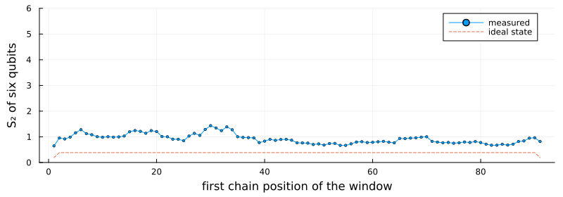
모든 윈도우가 이상적인 상태보다 약 0.5비트에서 1비트 정도 더 혼합되어 있으며, 노이즈가 가장 큰 구간은 사슬 위치 30~35 부근입니다. 최댓값 6에 가까운 윈도우가 없으므로 고장 난 큐비트는 없고, 분석에는 96큐비트 사슬 전체를 사용합니다. 일부 윈도우의 엔트로피가 6에 가까웠다면 그 윈도우들이 공유하는 큐비트를 제거하고, 그 큐비트 없이 사슬의 가장 긴 부분을 학습할 것입니다.
같은 순도가 CRM 사전 분포도 결정합니다. 각 윈도우에 대해 fitted_prior는 이상적인 상태를 가져와, 논문에서처럼 그 순도가 훈련 설정에서 측정된 순도와 일치하도록 국소 탈분극 세기를 피팅합니다.
다음 셀의 learn_and_validate 함수가 나머지 분석을 수행합니다. 훈련 설정으로 모델을 학습한 다음, 사슬의 처음 개 큐비트에 대해 12씩 늘려 가며 테스트 설정에서 와 를 추정합니다. 이는 논문의 그림 1(c,d)에 나오는 양입니다. 이상적인 상태는 기준선으로 같은 테스트 데이터에서 평가합니다.
이 셀은 로 함수를 실행한 다음 과 으로 반복하여, 학습 윈도우의 크기가 얼마나 중요한지 확인합니다. 본드 차원은 최대 이므로 은 곱 상태, 즉 큐비트 사이의 상관관계가 없는 각 큐비트 단독의 상태를 학습합니다.
function learn_and_validate(group; ideal, ell=2, k=3, sizes=12:12:group.N, seed=20260921, train_fraction=0.5)
    split = split_settings(group; seed, train_fraction)
    prior = fitted_prior(ideal, split.train)
    marginals = training_marginals(split.train; ell, prior)
    fit = learn_mpo(marginals, group.N; ell, maxbond=min(4, 4^ell), sweeps=20)
    last(fit.history).purity <= 1 ||
        @warn "The model has purity above one, so the fit diverged. Collect more settings or shots."
    statistics = afc_statistics(split.test, k; prior)
    learned = afc_prefix_curve(fit.model, statistics, split.test.NU; k, sizes)
    baseline = afc_prefix_curve(ideal, statistics, split.test.NU; k, sizes)
    model_entropy = [-log2(mpo_overlap(prefix_mpo(fit.model, n), prefix_mpo(fit.model, n))) for n in sizes]
    (; ell, fit, split, learned, baseline, model_entropy)
end

function plot_validation(results, title)
    n = [r.n for r in first(results).learned]
    # Marker, size, and line style per ℓ. The ℓ = 1 squares are small enough to sit inside the
    # ℓ = 2 circles, so both stay visible where the two curves overlap.
    style = Dict(2 => (:circle, 7, :solid), 1 => (:rect, 3.5, :dash), 0 => (:utriangle, 5, :dot))
    fidelity = plot(yscale=:log10, ylims=(1e-6, 1.5), legend=:bottomleft, xlabel="number of qubits N",
        ylabel="held-out F_max", title=title)
    entropy = plot(xlabel="number of qubits N", ylabel="Rényi-2 entropy S₂", legend=:topleft)
    held_out = first(results).learned
    # Draw every error bar before any marker, so the bars stay behind the symbols
    for (color, result) in enumerate(results)
        scatter!(fidelity, n, [r.fidelity for r in result.learned]; yerror=[r.fidelity_sem for r in result.learned],
            markersize=0, markerstrokecolor=color, label="")
    end
    scatter!(entropy, n, [r.entropy for r in held_out]; yerror=[r.entropy_sem for r in held_out],
        markersize=0, markerstrokecolor=:black, label="")
    for (color, result) in enumerate(results)
        marker, markersize, linestyle = style[result.ell]
        label = "learned model, ℓ = $(result.ell)"
        plot!(fidelity, n, [r.fidelity for r in result.learned]; color, marker, markersize, linestyle,
            markerstrokewidth=0, label)
        plot!(entropy, n, result.model_entropy; color, linestyle, linewidth=2, label)
    end
    plot!(fidelity, n, [r.fidelity for r in first(results).baseline]; marker=:diamond, markersize=5,
        linestyle=:dashdot, color=:black, label="ideal state")
    scatter!(entropy, n, [r.entropy for r in held_out]; marker=:circle, markersize=4, color=:black,
        label="held-out AFC estimate")
    plot(fidelity, entropy; layout=(1, 2), size=(1000, 400), left_margin=7Plots.mm, bottom_margin=7Plots.mm)
end

function summarize(result)
    final = last(result.learned)
    println("ℓ = ", result.ell, ", N = ", final.n, ": held-out F_max = ", round(final.fidelity, sigdigits=3), " ± ",
        round(final.fidelity_sem, sigdigits=2), " (ideal state: ", round(last(result.baseline).fidelity, sigdigits=2), ")")
    println("  S₂ = ", round(final.entropy, digits=2), " ± ", round(final.entropy_sem, digits=2),
        " held out; ", round(last(result.model_entropy), digits=2), " from the model")
    lowest = minimum(minimum(eigvals(Hermitian(operator_from_coefficients(local_coefficients(result.fit.model, w)))))
                     for w in unique(learning_windows(final.n, max(result.ell, 1))))
    println("  Most negative eigenvalue in any learning window: ", round(lowest, digits=4))
end

results_hw = [learn_and_validate(group_hw; ideal=ideal_hw, ell) for ell in (2, 1, 0)]
foreach(summarize, results_hw)
plot_validation(results_hw, "ibm_fez, 96-qubit chain")
ℓ = 2
, N = 96: held-out F_max = 0.591 ± 0.1 (ideal state: 0.0035)
  S₂ = 10.04 ± 0.28 held out; 10.21 from the model
  Most negative eigenvalue in any learning window: -0.0523
ℓ = 1, N = 96: held-out F_max = 0.554 ± 0.094 (ideal state: 0.0035)
  S₂ = 10.04 ± 0.28 held out; 10.26 from the model
  Most negative eigenvalue in any learning window: -0.0215
ℓ = 0, N = 96: held-out F_max = 6.18e-6 ± 1.1e-6 (ideal state: 0.0035)
  S₂ = 10.04 ± 0.28 held out; 32.01 from the model
  Most negative eigenvalue in any learning window: 0.0012
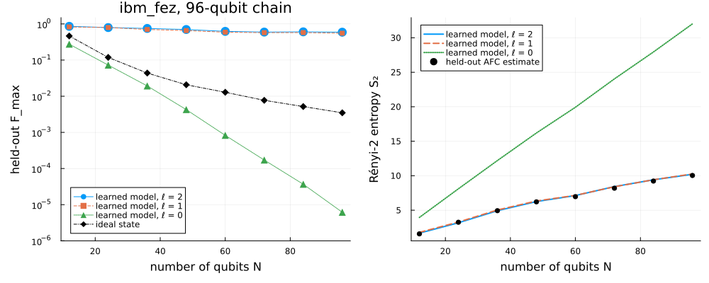
이 결과는 다른 프로세서에서 논문의 두 주장을 모두 재현합니다.
-
모델은 이상적인 상태보다 데이터를 훨씬 더 잘 설명합니다. 에서 모델의 보류 는 0.59 ± 0.10이며, 이상적인 상태는 0.0035입니다. 논문은
ibm_brisbane에서 약 0.75를 보고합니다. -
모델의 엔트로피는 모든 에서 테스트 데이터와 일치합니다. 에서 모델은 10.2, 테스트 데이터는 10.0 ± 0.3이며, 즉 으로, 이전 세대인
ibm_brisbane의 0.14~0.15와 비교됩니다.
윈도우 크기를 비교하면 정보가 어디에 있는지 알 수 있습니다. 이면 모델이 거의 그만큼 좋으므로(), 이 데이터에서는 몇 개 큐비트를 넘어서는 상관관계가 거의 도움이 되지 않습니다. 이면 곱 상태가 이웃한 큐비트 사이의 얽힘을 놓칩니다. 엔트로피는 10 대신 32까지 증가하고, 는 이상적인 상태보다도 더 빠르게 떨어져 에서 이 됩니다.
이 수치를 읽을 때는 다음 한계를 염두에 두세요.
-
훈련 분할. 오차 막대는 테스트 데이터의 통계 오차만 포함합니다. 같은 설정을 다른 방식으로 무작위 분할하면 , 에서 가 0.49에서 0.59 사이로 나옵니다.
-
마지막 sweep. 학습기는 항상 마지막 sweep의 모델을 반환하므로 테스트 데이터가 모델에 영향을 주지 않습니다.
-
양의 반정부호성. 모델은 양의 반정부호로 제한되지 않으며, 학습 윈도우에서 가장 작은 고유값은 약 입니다. 따라서 모델의 와 는 물리적 상태에 대해 보증된 성질이 아니라 하나의 연산자를 설명합니다.
-
인수분해. 보류한 모든 추정값은 AFC 가정에 의존하며, 이 가정은 측정 자체로는 보증할 수 없습니다.
다음 단계
-
깊이 2에 대한 논문의 매개변수(, 최대 본드 차원 8)로 깊이 2에서 실험을 반복하고, 학습기에 필요한 측정 설정의 수를 확인해 보세요.
-
대신 2-사이트 갱신(
training_marginals와learn_mpo의update=:two_site)으로 학습해 보세요. 이 방식은 매 단계 후 본드 차원을 절단하며, 훈련 설정이 더 적을 때 어떻게 동작하는지 살펴보세요. -
CRM 사전 분포 없이(
prior=nothing) 학습하고 보류 충실도를 비교해 보세요. -
저자들이 공개한
ibm_brisbane측정값에 같은 분석을 적용해 보세요. -
갱신과 AFC 추정량의 유도는 논문의 보충 자료를 읽어 보세요.
-
RandomMeas.jl예제에서 다른 무작위 측정 프로토콜을 살펴보세요.
참고 문헌
-
M. Votto, M. Ljubotina, C. Lancien, J. I. Cirac, P. Zoller, M. Serbyn, L. Piroli, and B. Vermersch, "Learning mixed quantum states in large-scale experiments", Phys. Rev. Lett. 136, 090801 (2026). arXiv:2507.12550
-
A. Elben, S. T. Flammia, H.-Y. Huang, R. Kueng, J. Preskill, B. Vermersch, and P. Zoller, "The randomized measurement toolbox", Nat. Rev. Phys. 5, 9 (2023). arXiv:2203.11374
-
H.-Y. Huang, R. Kueng, and J. Preskill, "Predicting many properties of a quantum system from very few measurements", Nat. Phys. 16, 1050 (2020). arXiv:2002.08953
-
A. Elben and B. Vermersch, "RandomMeas.jl: A Julia package for randomized measurements in quantum devices", Quantum 10, 2086 (2026). arXiv:2509.12749
-
B. Vermersch, A. Rath, B. Sundar, C. Branciard, J. Preskill, and A. Elben, "Enhanced estimation of quantum properties with common randomized measurements", PRX Quantum 5, 010352 (2024). arXiv:2304.12292
-
H. Zou, "Randomized measurements of a 96-qubit kicked-Ising state on ibm_fez", Zenodo (2026). doi:10.5281/zenodo.24116174