규모를 가로지르는 에르고딕성의 출현
이 노트북은 Onset of Ergodicity Across Scales on a Digital Quantum Processor [arXiv:2603.12236]의 실험을 실행하고 분석하는 방법을 단계별로 안내합니다. 모델에서 회로로, 비트열에서 엔트로피로, 노이즈가 있는 데이터에서 완화된 결과로, 그리고 16큐비트 시뮬레이션에서 IBM Quantum® Nighthawk 프로세서의 64큐비트 실행까지 다룹니다. 모든 코드가 여기에 있으며, 각 함수는 처음 필요한 곳에서 정의됩니다.
| 시간 | 섹션 |
|---|---|
| 0–1분 | 설정 |
| 1–6분 | 1. 모델에서 회로로 |
| 6–12분 | 2. 무엇을 측정하고 어떻게 추정할 것인가 |
| 12–19분 | 3. 노이즈와 그 제거 방법 |
| 19–24분 | 4. 대규모 실행 |
| 24–33분 | 5. 하드웨어 데이터 |
| 33–35분 | 마무리 |
따라 하기. 셀을 위에서 아래로 순서대로 실행하세요. IBM Quantum 계정은 필요하지 않습니다. 하드웨어 작업을 제출하는 셀은 꺼져 있으며, 5번 섹션에서는 저장된 하드웨어 실행을 분석합니다. 이 실행은 설정 셀이 data/에 내려받습니다. 토론용 질문은 질문으로 표시되어 있으니, 답을 열어 보기 전에 먼저 답해 보세요.
설정
Python 3.12 이상과 다음 패키지가 필요합니다.
-
Qiskit SDK v2.5 이상, 시각화 지원 포함
-
Qiskit Runtime v0.49 이상(
pip install qiskit-ibm-runtime) -
Qiskit Aer v0.17 이상(
pip install qiskit-aer) -
Samplomatic v0.21 이상(
pip install samplomatic) -
NumPy와 Matplotlib
설정 셀은 저장된 하드웨어 실행과 MPS 참조(약 9 MB)도 data/에 내려받습니다. 이미 있는 경우에는 내려받지 않습니다.
# Added by doQumentation — installs the packages this notebook needs if they are missing
import importlib.util

_needed = {"matplotlib": "matplotlib", "numpy": "numpy", "qiskit": "qiskit", "qiskit_aer": "qiskit-aer", "qiskit_ibm_runtime": "qiskit-ibm-runtime", "samplomatic": "samplomatic"}
_missing = [pip for module, pip in _needed.items()
            if importlib.util.find_spec(module) is None]
# One at a time, so a package that fails to install does not block the others
for _pip in _missing:
    %pip install -q {_pip}
if not _missing:
    print("\u2713 All required packages are installed")
from math import comb
from pathlib import Path
from urllib.request import urlretrieve

import matplotlib.pyplot as plt
import numpy as np
from qiskit import ClassicalRegister, QuantumCircuit, QuantumRegister
from qiskit.primitives import StatevectorSampler
from qiskit.quantum_info import (
    PauliLindbladMap,
    QubitSparsePauli,
    Statevector,
)
from qiskit.transpiler import generate_preset_pass_manager
from qiskit_aer import AerSimulator
from qiskit_aer.noise import NoiseModel, ReadoutError, depolarizing_error
from qiskit_aer.primitives import SamplerV2 as AerSampler

RUN_ON_HARDWARE = (
    False  # True submits the 8x8 jobs in section 4 (needs Nighthawk access)
)
COMPUTE_MPS_REFERENCES = False  # True recomputes the MPS references in section 5 (about 18 minutes)

# Download the saved hardware run and MPS references, unless they are already in data/
data_url = "https://raw.githubusercontent.com/Qiskit/documentation/main/datasets/tutorials/onset-of-ergodicity"
Path("data").mkdir(exist_ok=True)
for name in ("hardware_run.npz", "mps_references_all.npz"):
    if not Path("data", name).exists():
        urlretrieve(f"{data_url}/{name}", Path("data", name))
1. 모델에서 회로로
2큐비트 게이트
격자의 모든 결합 에는 하이젠베르크 얽힘 연산 뒤에 무작위 장이 이어지는 동일한 2큐비트 게이트가 적용됩니다.
여기서 는 모든 게이트마다 에서 균등하게 뽑습니다.
질문. 를 하드웨어가 실행할 수 있는 게이트로 어떻게 분해하겠습니까?
정답
장(field) 부분은 쉽습니다. 는 각 큐비트에 대한 단일 큐비트 회전 입니다.
얽힘 연산 부분이 어려운 부분입니다. , , 는 서로 교환하므로 세 개의 회전 , , 로 분해됩니다. 각각 CNOT이 두 개 필요하므로 게이트당 CNOT은 여섯 개가 됩니다.
더 나은 방법이 있습니다. 모든 2큐비트 게이트는 최대 세 개의 CNOT과 단일 큐비트 회전으로 만들 수 있습니다. 최적 회로는 형태에서 출발하며, 이 얽힘 연산은 로 이미 그 형태입니다. 따라서 세 개의 CNOT에 바로 대응되고, 단일 큐비트 각도는 에 대해 선형입니다. 실험 코드는 이 방식으로 게이트를 만듭니다.
하드웨어에서는 2큐비트 게이트마다 노이즈가 더해지므로 CNOT 수를 절반으로 줄이는 것이 중요합니다.
def xxyyzz_gate(circuit, coupling, i, j):
    # exp(iJ(XX + YY + ZZ)) with three CNOTs; only the rotation angles depend on J
    circuit.rz(-np.pi / 2, j)
    circuit.cx(j, i)
    circuit.rz(np.pi / 2 - 2 * coupling, i)
    circuit.ry(2 * coupling - np.pi / 2, j)
    circuit.cx(i, j)
    circuit.ry(np.pi / 2 - 2 * coupling, j)
    circuit.cx(j, i)
    circuit.rz(np.pi / 2, i)

def heisenberg_gate(circuit, coupling, i, j, h_i, h_j):
    # The entangler first, then the random fields exp(i h Z)
    xxyyzz_gate(circuit, coupling, i, j)
    circuit.rz(-2 * h_i, i)
    circuit.rz(-2 * h_j, j)

h_i, h_j = 0.3, -0.7
gate = QuantumCircuit(2)
heisenberg_gate(gate, 0.05 * np.pi, 0, 1, h_i, h_j)
gate.draw("mpl")

벽돌 배열과 Floquet 주기
게이트는 겹치지 않는 결합으로 이루어진 네 개의 서브레이어로 정사각 격자를 채우며, 이를 벽돌 배열이라고 합니다. 짝수 열에서 시작하는 가로 결합, 홀수 열에서 시작하는 가로 결합, 짝수 행에서 시작하는 세로 결합, 홀수 행에서 시작하는 세로 결합의 순서입니다. 큐비트 는 사이트 에 위치합니다.
def brickwork_layers(num_cols, num_rows):
    # Bonds of the square lattice, in the four sublayers of the brickwork
    def qubit(x, y):
        return y * num_cols + x

    layers = []
    for p in (0, 1):  # horizontal bonds starting on even, then odd, columns
        layers.append(
            [
                (qubit(x, y), qubit(x + 1, y))
                for y in range(num_rows)
                for x in range(p, num_cols - 1, 2)
            ]
        )
    for p in (0, 1):  # vertical bonds starting on even, then odd, rows
        layers.append(
            [
                (qubit(x, y), qubit(x, y + 1))
                for y in range(p, num_rows - 1, 2)
                for x in range(num_cols)
            ]
        )
    return layers

brickwork_layers(4, 4)
[[(0, 1), (2, 3), (4, 5), (6, 7), (8, 9), (10, 11), (12, 13), (14, 15)],
 [(1, 2), (5, 6), (9, 10), (13, 14)],
 [(0, 4), (1, 5), (2, 6), (3, 7), (8, 12), (9, 13), (10, 14), (11, 15)],
 [(4, 8), (5, 9), (6, 10), (7, 11)]]
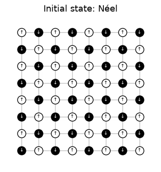
네 개의 서브레이어가 하나의 Floquet 주기를 이룹니다. 이 주기는 동일한 장으로 번 반복되므로, 동역학은 공간적으로는 무작위이고 시간적으로는 주기적입니다. 회로는 Néel 상태에서 시작하며, 는 격자 한 변 길이의 절반입니다. 다음 셀은 논문의 그림 5 스타일로, 하드웨어 실행에 사용된 장을 적용하여 하드웨어 격자의 Floquet 주기 하나를 서브레이어별로 그립니다. 굵은 결합이 각 서브레이어의 게이트입니다. 게이트가 작용하는 각 큐비트는 이후에 받는 무작위 장 에 따라 색이 칠해지고, 유휴 큐비트는 흰색입니다. 화살표는 Néel 초기 상태를 나타내며, 는 입니다. 논문의 그림은 세로 서브레이어를 먼저 적용하는데, 어느 순서든 물리적 결과는 달라지지 않을 것으로 예상됩니다.
# circuit structure, 8x8 system:
side = 8
all_bonds = [bond for layer in brickwork_layers(side, side) for bond in layer]

# get the disorder parameters for a given system:
def sample_disorder(num_cols, num_rows, rng):
    # One pair of fields (h_i, h_j) per gate, reused in every Floquet cycle
    return [
        [
            (bond, tuple(rng.uniform(-np.pi / 2, np.pi / 2, 2)))
            for bond in layer
        ]
        for layer in brickwork_layers(num_cols, num_rows)
    ]

# build the structure for the 8x8 system
example_disorder = sample_disorder(
    side, side, np.random.default_rng(7)
)  # the hardware fields (section 4)
titles = [
    r"$U^H_\mathrm{even}$",
    r"$U^H_\mathrm{odd}$",
    r"$U^V_\mathrm{even}$",
    r"$U^V_\mathrm{odd}$",
]
norm = plt.Normalize(-np.pi / 2, np.pi / 2)
cmap = plt.get_cmap("RdBu_r")

fig, axes = plt.subplots(1, 4, figsize=(16, 4.8), layout="constrained")
for ax, title, sublayer in zip(axes, titles, example_disorder):
    for i, j in all_bonds:
        ax.plot(
            [i % side, j % side],
            [i // side, j // side],
            color="0.75",
            lw=1,
            zorder=0,
        )
    fields = {}
    for (i, j), (h_i, h_j) in sublayer:
        ax.plot(
            [i % side, j % side],
            [i // side, j // side],
            color="0.2",
            lw=4,
            zorder=1,
        )
        fields[i], fields[j] = h_i, h_j
    for q in range(side * side):
        x, y = q % side, q // side
        ax.scatter(
            x,
            y,
            s=260,
            color=cmap(norm(fields[q])) if q in fields else "white",
            edgecolor="black",
            zorder=2,
        )
        ax.text(
            x,
            y,
            "↓" if (x + y) % 2 else "↑",
            ha="center",
            va="center",
            fontsize=9,
            zorder=3,
        )
    ax.set_aspect("equal")
    ax.set_xlim(-1, side)  # padding, so the panels read as separate steps
    ax.set_ylim(side, -1)
    ax.axis("off")
    ax.set_title(title, y=-0.1, fontsize=13)
fig.colorbar(
    plt.cm.ScalarMappable(norm=norm, cmap=cmap),
    ax=axes,
    shrink=0.7,
    label="Field $h$ after the gate",
)
plt.show()
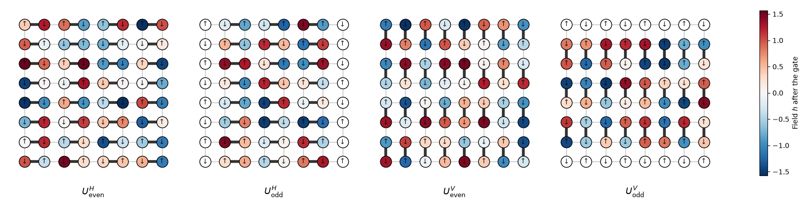
초기 상태를 정의합니다.
# initial state
def neel_state(circuit, num_cols, num_rows, layout):
    for y in range(num_rows):
        for x in range(num_cols):
            if (x + y) % 2 == 1:
                circuit.x(layout[y * num_cols + x])
# The initial Néel state: |1⟩ (black, ↓) on odd sites, |0⟩ (white, ↑) on even sites

fig, ax = plt.subplots(figsize=(4, 4.4))
for i, j in all_bonds:
    ax.plot(
        [i % side, j % side],
        [i // side, j // side],
        color="0.75",
        lw=1,
        zorder=0,
    )
for q in range(side * side):
    x, y = q % side, q // side
    excited = (x + y) % 2 == 1
    ax.scatter(
        x,
        y,
        s=150,
        color="black" if excited else "white",
        edgecolor="black",
        zorder=2,
    )
    ax.text(
        x,
        y,
        "↓" if excited else "↑",
        ha="center",
        va="center",
        fontsize=7,
        color="white" if excited else "black",
        zorder=3,
    )
ax.set_aspect("equal")
ax.set_xlim(-1, side)
ax.set_ylim(side, -1)
ax.axis("off")
ax.set_title("Initial state: Néel", fontsize=13)
plt.show()
# actual circuit construction:
def heisenberg_floquet_circuit(
    num_cols, num_rows, coupling, num_cycles, disorder, measure=True
):
    num_qubits = num_cols * num_rows
    circuit = QuantumCircuit(num_qubits)
    neel_state(circuit, num_cols, num_rows, list(range(num_qubits)))
    cycle = QuantumCircuit(num_qubits)
    for sublayer in disorder:
        for (i, j), (h_i, h_j) in sublayer:
            heisenberg_gate(cycle, coupling, i, j, h_i, h_j)
    for _ in range(num_cycles):
        circuit.compose(cycle, inplace=True)
    if measure:
        circuit.measure_all()
    return circuit
예제
시뮬레이션은 두 주기의 격자와 논문에서 연구한 결합 을 사용합니다. 하나의 장 집합을 모든 결합에 재사용합니다.
# simulation parameters:
num_cols = num_rows = 4
num_qubits = num_cols * num_rows
num_cycles = 2
couplings = (
    np.array([0.005, 0.01, 0.02, 0.03, 0.04, 0.05, 0.06, 0.08, 0.10, 0.125])
    * np.pi
)
disorder = sample_disorder(num_cols, num_rows, np.random.default_rng(42))

# circuit construction:
logical_circuits = [
    heisenberg_floquet_circuit(
        num_cols, num_rows, coupling, num_cycles, disorder
    )
    for coupling in couplings
]
logical_circuits[5].draw(output="mpl", fold=-1)

# transpiling the circuit:
pass_manager = generate_preset_pass_manager(
    optimization_level=3,
    basis_gates=["cz", "rz", "sx", "x"],
    seed_transpiler=7,
)
circuits = [pass_manager.run(circuit) for circuit in logical_circuits]

def two_qubit_stats(circuit):
    count = sum(1 for inst in circuit.data if inst.operation.num_qubits == 2)
    depth = circuit.depth(lambda inst: inst.operation.num_qubits == 2)
    return count, depth

stats = {two_qubit_stats(circuit) for circuit in circuits}
assert len(stats) == 1, "the CZ structure should not depend on J"
num_cz, depth = stats.pop()
print(
    f"{num_qubits} qubits: {num_cz} CZ gates in {depth} layers, for every coupling"
)
circuits[5].draw("mpl", fold=-1, scale=0.4)
16 qubits: 144 CZ gates in 24 layers, for every coupling

회로(와 실험)가 IBM Nighthawk에 맞게 설계되었으므로 영리한 컴파일러는 필요하지 않습니다.
격자 시뮬레이션
격자에서는 두 가지를 모두 할 수 있습니다. 모든 결합에서 정확한 상태를 계산하고, 실험과 마찬가지로 모든 회로를 10,000샷으로 샘플링합니다. 샷은 (배치, 샷, 큐비트) 형태로 저장되며, 이는 하드웨어 데이터의 무작위화와 같은 레이아웃입니다. 여기서는 10,000샷 전체가 하나의 배치이므로 배치에 대한 부트스트랩은 샷 노이즈를 더하지 않으며, 다음 플롯의 오차 막대는 주변 분포 위치 간의 퍼짐만 보여 줍니다.
exact_states = [
    Statevector(
        heisenberg_floquet_circuit(
            num_cols, num_rows, c, num_cycles, disorder, measure=False
        )
    )
    for c in couplings
]

shots = 10_000
results = (
    StatevectorSampler(default_shots=shots, seed=1234).run(circuits).result()
)

# the output of the simulation for the 10 couplings
bits = [
    result.data.meas.to_bool_array(order="little").reshape(
        1, 10_000, num_qubits
    )
    for result in results
]

print(bits[0])
[[[False  True False ... False  True False]
  [False  True False ... False  True False]
  [False  True False ... False  True False]
  ...
  [False  True False ... False  True False]
  [False  True False ... False  True False]
  [False  True False ... False  True False]]]
2. 무엇을 측정하고 어떻게 추정할 것인가
IPR과 충돌 엔트로피
비트열 분포가 인 개 큐비트의 주변 분포 에 대해, 추정할 양은 주변 분포의 역참여비(IPR)이며, 이로부터 충돌 엔트로피를 얻습니다.
는 두 샷이 주변 분포에서 일치할 확률이기도 합니다. 곱 상태는 이고 무작위 상태는 이므로, 주변 분포가 무작위에 가까워질수록 는 0에서 약 비트까지 올라갑니다.
추정기 1: 샷 쌍 세기
질문. 샷으로부터 이 양을 어떻게 추정하겠습니까?
정답
단순한 추정기는 샷에서 각 를 으로 계산한 다음 을 합산합니다. 이 추정기는 편향되어 있습니다.
은 모든 샷이 자기 자신과 일치하는 것으로 세기 때문에 추정값이 높아집니다. 평균적으로 대신 을 줍니다. 는 두 샷이 일치할 확률이므로 서로 다른 샷의 쌍만 세세요.
이 추정기는 편향이 없으며, 아래의 ipr_from_shots가 계산하는 것이 바로 이것입니다.
# IPR expectation values:

# refactor this function cause it does not scale
def ipr_from_shots(bits):
    # Pair-counting estimate of the IPR of a marginal: the fraction of pairs of different shots
    # that agree on it. bits holds the marginal's qubits only, with shape (randomizations, shots,
    # qubits), and all randomizations are pooled.
    n = bits.shape[-1]
    outcomes = bits @ 2 ** np.arange(
        n
    )  # each shot's marginal bitstring, read as an integer
    counts = np.bincount(outcomes.ravel())  # how often each outcome occurs
    total = counts.sum()
    return float((counts * (counts - 1)).sum() / (total * (total - 1)))

def collision_entropy(ipr):
    return -np.log2(ipr)
추정기 2: Parseval 전개
IPR은 주변 분포의 비어 있지 않은 모든 부분집합 의 패리티 를 통해서도 쓸 수 있습니다.
PEA 같은 오류 완화 방법은 확률이 아니라 기댓값에 대해 작동하기 때문에 이 형태가 중요합니다. 큐비트 하나: 결과 확률은 이고 이므로,
주변 분포: 큐비트에 라는 이름을 붙이면, 주변 분포에는 개의 패리티가 있습니다. 단일 큐비트 4개, 쌍 6개, 삼중항 4개, 그리고 주변 분포 전체이므로,
def parity_supports(patch):
    # All nonempty subsets S of the marginal
    return sorted(
        [
            tuple(q for k, q in enumerate(patch) if mask & (1 << k))
            for mask in range(1, 1 << len(patch))
        ],
        key=len,
    )

def parity_expectation_values(bits, supports):
    # Shot-averaged <Z_S> for every support, per randomization
    signs = 1 - 2 * bits.astype(np.int8)
    return np.stack(
        [signs[..., list(s)].prod(axis=-1).mean(axis=-1) for s in supports],
        axis=-1,
    )

# Example: the parities of a 3-qubit marginal made of lattice qubits 5, 6, and 9
print(parity_supports([5, 6, 9]))
print(f"A 3×3 marginal has {len(parity_supports(range(9)))} parities")
[(5,), (6,), (9,), (5, 6), (5, 9), (6, 9), (5, 6, 9)]
A 3×3 marginal has 511 parities
주변 분포에 대한 평균
유용한 추가 함수: Haar 값, 주변 분포 선택, 부트스트래핑, 평균화.
# functions for the Haar values on plots:
def haar_ipr(num_patch, num_qubits):
    # Mean IPR of a marginal for Haar-random states in the sector with num_qubits // 2 ones
    weight = num_qubits // 2
    dimension = comb(num_qubits, weight)
    total = 0
    for k in range(num_patch + 1):  # k ones on the marginal
        rest = (
            comb(num_qubits - num_patch, weight - k) if weight - k >= 0 else 0
        )
        total += comb(num_patch, k) * rest * (rest + 1)
    return total / (dimension * (dimension + 1))

def haar_entropy(num_patch, num_qubits):
    return collision_entropy(haar_ipr(num_patch, num_qubits))

# definitions of positions in the lattice:
def patch_qubits(anchor, shape, num_cols):
    # Lattice indices of a rectangular marginal with its top-left corner at anchor
    (x0, y0), (width, height) = anchor, shape
    return [
        (y0 + dy) * num_cols + (x0 + dx)
        for dy in range(height)
        for dx in range(width)
    ]

def all_positions(shape, num_cols, num_rows):
    # Every placement of a (width, height) marginal on the lattice
    width, height = shape
    return [
        patch_qubits((x, y), shape, num_cols)
        for y in range(num_rows - height + 1)
        for x in range(num_cols - width + 1)
    ]

# bootstrapping for error bars:
bootstrap_rng = np.random.default_rng(0)

def bootstrap_error(statistic, *samples, axis=0, num_resamples=50):
    # Shot noise of a statistic, from resampling the randomizations (along axis of every
    # sample) with replacement
    values = []
    for _ in range(num_resamples):
        resampled = [
            np.take(
                x,
                bootstrap_rng.integers(0, x.shape[axis], x.shape[axis]),
                axis=axis,
            )
            for x in samples
        ]
        values.append(statistic(*resampled))
    return float(np.std(values, ddof=1))

# averaging the ipr over marginals:
def average_ipr(iprs, shot_errors):
    # iprs and shot_errors have shape (positions, couplings). The mean IPR over positions, and its
    # error: the spread between positions plus the shot noise of each (law of total variance)
    iprs, shot_errors = np.asarray(iprs), np.asarray(shot_errors)
    count = len(iprs)
    variance = (
        iprs.var(axis=0, ddof=1) / count
        + (shot_errors**2).sum(axis=0) / count**2
    )
    return iprs.mean(axis=0), np.sqrt(variance)
# Calculating exact simulation entropies:
patch_shapes = {
    "1×1": (1, 1),
    "1×2": (2, 1),
    "2×2": (2, 2),
    "2×3": (3, 2),
    "3×3": (3, 3),
}

# calculate the exact entropies:
sim_positions = {
    label: all_positions(shape, num_cols, num_rows)
    for label, shape in patch_shapes.items()
}
exact_iprs = {  # shape (positions, couplings)
    label: np.array(
        [
            [(s.probabilities(qargs=q) ** 2).sum() for s in exact_states]
            for q in qubit_lists
        ]
    )
    for label, qubit_lists in sim_positions.items()
}
exact_entropies = {
    label: collision_entropy(v.mean(axis=0))
    for label, v in exact_iprs.items()
}

# Average IPR of every shape over its positions, from the sampled shots, then the entropy
iprs_from_shots = {}  # per shape: average IPR and its error, at every coupling
entropies_from_shots = {}  # per shape: average entropy and its error, at every coupling
for label, qubit_lists in sim_positions.items():
    iprs = [[ipr_from_shots(b[:, :, q]) for b in bits] for q in qubit_lists]

    # bootstrapping over subsampling for error bars:
    errors = [
        [bootstrap_error(ipr_from_shots, b[:, :, q]) for b in bits]
        for q in qubit_lists
    ]
    ipr, ipr_error = average_ipr(iprs, errors)
    iprs_from_shots[label] = (ipr, ipr_error)
    entropies_from_shots[label] = (
        collision_entropy(ipr),
        ipr_error / (ipr * np.log(2)),
    )
# Now plot the average IPR on the left, and the same averages as entropies on the right
colors = plt.cm.plasma(np.linspace(0.05, 0.8, len(patch_shapes)))
fig, (ax_ipr, ax_entropy) = plt.subplots(1, 2, figsize=(12.8, 4.2))
for (label, qubit_lists), color in zip(sim_positions.items(), colors):
    n = len(qubit_lists[0])
    ipr, ipr_error = iprs_from_shots[label]
    entropy, entropy_error = entropies_from_shots[label]
    # Left: the average IPR, with its exact value and its random-state value
    ax_ipr.axhline(haar_ipr(n, num_qubits), color=color, ls="dashdot", lw=0.9)
    ax_ipr.plot(
        couplings / np.pi, exact_iprs[label].mean(axis=0), color=color
    )
    ax_ipr.errorbar(
        couplings / np.pi,
        ipr,
        yerr=ipr_error,
        fmt="o",
        color=color,
        mec="white",
        ms=7,
        capsize=3,
        label=f"{label} ({len(qubit_lists)} positions)",
    )
    # Right: the average collision entropy
    ax_entropy.axhline(
        haar_entropy(n, num_qubits), color=color, ls="dashdot", lw=0.9
    )
    ax_entropy.plot(couplings / np.pi, exact_entropies[label], color=color)
    ax_entropy.errorbar(
        couplings / np.pi,
        entropy,
        yerr=entropy_error,
        fmt="o",
        color=color,
        mec="white",
        ms=7,
        capsize=3,
        label=f"{label} ({len(qubit_lists)} positions)",
    )
ax_ipr.set_yscale("log")
ax_ipr.set_ylabel("Average IPR")
ax_entropy.set_ylabel("Average collision entropy (bits)")
for ax in (ax_ipr, ax_entropy):
    ax.set_xlabel("Coupling $J/\\pi$")
fig.suptitle("Exact (lines) and sampled (dots), 4×4 lattice, 2 cycles")
ax_entropy.legend(title="Marginal", loc="upper left")
fig.tight_layout()
plt.show()
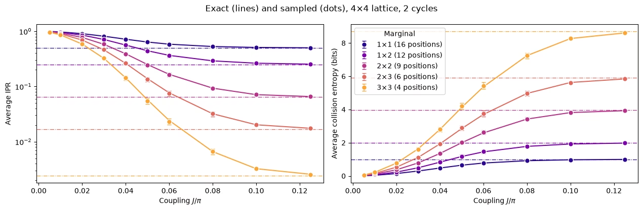
모든 주변 분포 형태는 무작위 상태의 값을 향해 매끄럽게 상승하며, 더 큰 주변 분포는 더 큰 에서 그 값에 도달합니다.
3. 노이즈와 그 제거 방법
노이즈가 있는 시뮬레이션
이제 노이즈를 추가합니다. 모든 CZ 게이트에 1% 2큐비트 탈분극 노이즈를, 모든 큐비트에 3% 판독 오류를 적용하고 Qiskit Aer sampler로 샘플링합니다. 회로에 CZ 게이트가 144개이므로 8×8 하드웨어 회로가 겪는 노이즈보다 훨씬 적지만, 노이즈의 영향을 확인하기에는 충분합니다. 시뮬레이션은 여섯 개의 결합과 각각 4,000샷을 사용하며 약 1.5분이 걸립니다.
질문. 실행하기 전에 예상해 보세요. 노이즈가 있으면 시스템이 더 열평형화된 것처럼 보일까요, 덜 열평형화된 것처럼 보일까요?
정답
더 그렇게 보입니다. 노이즈는 결과를 뒤섞어 모든 주변 분포를 균일한 분포 쪽으로 밀어 내므로 원시 IPR은 떨어지고 엔트로피는 올라갑니다. 완화하지 않으면 노이즈는 실제로 없는 열평형화처럼 보이고, 교차점도 너무 일찍 나타납니다.
# define the noise model

noise_model = NoiseModel()
# two qubit depolarizing noise:
noise_model.add_all_qubit_quantum_error(depolarizing_error(0.01, 2), ["cz"])
# symmetric readout noise:
noise_model.add_all_qubit_readout_error(
    ReadoutError([[0.97, 0.03], [0.03, 0.97]])
)

# simulation is done using trajectories
noisy_sampler = AerSampler(
    default_shots=4000,
    seed=1,
    options={"backend_options": {"noise_model": noise_model}},
)

# choose a subset of J values for speed:
noisy_indices = [
    0,
    2,
    3,
    5,
    7,
    9,
]  # J/π = 0.005, 0.02, 0.03, 0.05, 0.08, 0.125
noisy_results = noisy_sampler.run(
    [circuits[k] for k in noisy_indices]
).result()

# No twirling here, so the 20 "randomizations" are just batches of 200 shots
noisy_bits = {
    k: result.data.meas.to_bool_array(order="little").reshape(
        20, 200, num_qubits
    )
    for k, result in zip(noisy_indices, noisy_results)
}
# Calculating noisy entropies

# Average IPR of every shape over its positions, from the noisy shots, then the entropy
noisy_iprs = {}  # per shape: average IPR and its error, at every noisy coupling
noisy_entropies = {}  # per shape: average entropy and its error, at every noisy coupling
for label, qubit_lists in sim_positions.items():
    iprs = [
        [ipr_from_shots(noisy_bits[k][:, :, q]) for k in noisy_indices]
        for q in qubit_lists
    ]

    # bootstrapping over subsampling for error bars:
    errors = [
        [
            bootstrap_error(ipr_from_shots, noisy_bits[k][:, :, q])
            for k in noisy_indices
        ]
        for q in qubit_lists
    ]
    ipr, ipr_error = average_ipr(iprs, errors)
    noisy_iprs[label] = (ipr, ipr_error)
    noisy_entropies[label] = (
        collision_entropy(ipr),
        ipr_error / (ipr * np.log(2)),
    )
fig, (ax_ipr, ax_entropy) = plt.subplots(1, 2, figsize=(12.8, 4.2))
for (label, qubit_lists), color in zip(sim_positions.items(), colors):
    n = len(qubit_lists[0])
    ipr, ipr_error = noisy_iprs[label]
    entropy, entropy_error = noisy_entropies[label]
    # Left: the average IPR, with its exact value and its random-state value
    ax_ipr.axhline(haar_ipr(n, num_qubits), color=color, ls="dashdot", lw=0.9)
    ax_ipr.plot(
        couplings / np.pi, exact_iprs[label].mean(axis=0), color=color
    )
    ax_ipr.errorbar(
        couplings[noisy_indices] / np.pi,
        ipr,
        yerr=ipr_error,
        fmt="o",
        color=color,
        mec="white",
        ms=7,
        capsize=3,
        label=label,
    )
    # Right: the same averages as entropies
    ax_entropy.axhline(
        haar_entropy(n, num_qubits), color=color, ls="dashdot", lw=0.9
    )
    ax_entropy.plot(couplings / np.pi, exact_entropies[label], color=color)
    ax_entropy.errorbar(
        couplings[noisy_indices] / np.pi,
        entropy,
        yerr=entropy_error,
        fmt="o",
        color=color,
        mec="white",
        ms=7,
        capsize=3,
        label=label,
    )
ax_ipr.set_yscale("log")
ax_ipr.set_ylabel("Average IPR")
ax_entropy.set_ylabel("Average collision entropy (bits)")
for ax in (ax_ipr, ax_entropy):
    ax.set_xlabel("Coupling $J/\\pi$")
fig.suptitle("Exact (lines) and noisy raw estimates (dots)")
ax_entropy.legend(title="Marginal", loc="lower right")
fig.tight_layout()
plt.show()
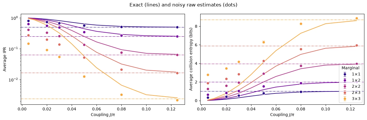
브레인스토밍: 이를 어떻게 되돌리겠습니까?
제안하는 접근법
작은 에서는 상태가 거의 얽혀 있지 않으므로 64큐비트라도 이상적인 답을 고전적으로 계산하는 비용이 낮습니다. 따라서 작은 보정 결합 에서 노이즈의 영향을 측정하고 이를 이용해 다른 모든 결합을 보정하는 방법을 생각할 수 있습니다. 이를 저얽힘 보정(low-entanglement calibration, LEC)이라 하며, 자연스러운 방법이 두 가지 있습니다.
IPR에 대한 LEC. IPR이 균일 분포의 값 를 넘는 초과분을 주변 분포마다 하나의 인수로 재조정합니다.
기댓값에 대한 LEC. 주변 분포의 모든 패리티를 각자의 인수로 재조정한 다음 Parseval 공식으로 IPR을 다시 구성합니다.
코드에서는 2번 섹션에서처럼 재조정된 각 패리티의 제곱에서 분산을 빼서 편향을 제거합니다.
모든 가 과 같다면 두 방법은 동일합니다.
Question. What are the pros and cons of these methods?
정답
Pros
-
저렴함: 장치에서 추가 데이터가 필요 없고 에서의 고전 시뮬레이션만 필요합니다.
-
회로의 구조를 활용함: 회로 깊이와 CZ 레이어는 에 따라 변하지 않으므로, 에서의 노이즈는 다른 모든 에서의 노이즈와 같습니다.
Cons
- 관측량에 대한 노이즈의 영향이 에 의존하지 않는다고 가정함: 노이즈 자체는 같지만, 그것이 IPR이나 각 를 감쇠시키는 방식은 가 커짐에 따라 달라질 수 있습니다.
노이즈가 있는 시뮬레이션에서 두 방법 비교
# function to mitigate the IPR signal:
def mitigate_ipr_w_lec(
    ipr_raw, ipr_raw_calibration, ipr_ideal_calibration, num_patch
):
    # LEC on the IPR: one factor R0 for the excess over the uniform value
    uniform = 2.0**-num_patch
    factor = (ipr_ideal_calibration - uniform) / (
        ipr_raw_calibration - uniform
    )
    return uniform + factor * (ipr_raw - uniform)

# function used to calculate the target <Z> expectation values
def parities_from_probabilities(probabilities):
    # Ideal <Z_S> from a marginal distribution, in parity_supports order: subsets
    # by size, and in bitmask order within each size
    outcomes = np.arange(len(probabilities))
    masks = np.array(sorted(range(1, len(probabilities)), key=int.bit_count))
    signs = (-1.0) ** np.bitwise_count(outcomes[:, None] & masks[None, :])
    return np.asarray(probabilities) @ signs

# calculate boosting factors:
def lec_z_factors(calibration_parities, ideal_parities):
    # LEC on <Z>: one factor r_S per parity, from data with shape (randomizations, supports).
    return ideal_parities / calibration_parities.mean(axis=0)

# function to mitigate the IPR from <Z> expectation values:
def mitigate_ipr_w_lec_on_parities(
    parities, calibration_parities, ideal_calibration_parities, num_patch
):
    # LEC on <Z>: rescale each parity by its factor r_S = ideal / raw at J0, then rebuild the IPR
    # with Parseval. parities and calibration_parities have shape (randomizations, supports).
    # Each squared, rescaled parity is debiased by subtracting its variance, which to first
    # order combines the shot noise at J. The shot noise of r_S from J0 is omitted; including it
    # does not change the results.
    factors = lec_z_factors(calibration_parities, ideal_calibration_parities)
    mean = parities.mean(axis=0)  # mean over the twirling instances
    variance = parities.var(axis=0, ddof=1) / len(
        parities
    )  # variance of the mean
    rescaled = factors * mean
    rescaled_variance = factors**2 * variance
    return float((1 + np.sum(rescaled**2 - rescaled_variance)) / 2**num_patch)
def lec_estimates(patch_bits, parities, ideal, calibration, num_patch):
    # LEC on the IPR and on <Z> for one marginal position, at every coupling: values and shot
    # noise. patch_bits (the bits of the marginal only) and parities are per coupling, with
    # randomizations first.
    q_ideal = (ideal**2).sum()
    ideal_parities = parities_from_probabilities(ideal)

    def ipr_statistic(b, c):
        return mitigate_ipr_w_lec(
            ipr_from_shots(b), ipr_from_shots(c), q_ideal, num_patch
        )

    def z_statistic(p, c):
        return mitigate_ipr_w_lec_on_parities(p, c, ideal_parities, num_patch)

    values = {"LEC on IPR": [], "LEC on ⟨Z⟩": []}
    errors = {"LEC on IPR": [], "LEC on ⟨Z⟩": []}
    for k in range(len(patch_bits)):
        if (
            k == calibration
        ):  # both match the ideal value at J0 by construction
            for method in values:
                values[method].append(q_ideal)
                errors[method].append(0.0)
            continue
        values["LEC on IPR"].append(
            ipr_statistic(patch_bits[k], patch_bits[calibration])
        )
        errors["LEC on IPR"].append(
            bootstrap_error(
                ipr_statistic, patch_bits[k], patch_bits[calibration]
            )
        )
        values["LEC on ⟨Z⟩"].append(
            z_statistic(parities[k], parities[calibration])
        )
        errors["LEC on ⟨Z⟩"].append(
            bootstrap_error(z_statistic, parities[k], parities[calibration])
        )
    return values, errors

# getting all the data:
calibration_index = 0  # index of J0 = 0.005π in noisy_indices
mitigated = {
    "LEC on IPR": {},
    "LEC on ⟨Z⟩": {},
}  # per shape: (values, errors), each (positions, couplings)
for label, qubit_lists in sim_positions.items():
    n = len(qubit_lists[0])
    per_position = []
    for qubits in qubit_lists:
        supports = parity_supports(qubits)
        parities = [
            parity_expectation_values(noisy_bits[k], supports)
            for k in noisy_indices
        ]
        patch_bits = [noisy_bits[k][:, :, qubits] for k in noisy_indices]
        ideal = exact_states[noisy_indices[calibration_index]].probabilities(
            qargs=qubits
        )
        per_position.append(
            lec_estimates(patch_bits, parities, ideal, calibration_index, n)
        )
    for method in mitigated:
        mitigated[method][label] = (
            [p[0][method] for p in per_position],
            [p[1][method] for p in per_position],
        )

# Average over positions, then the entropy, for both methods
mitigated_entropies = {
    method: {} for method in mitigated
}  # per method and shape: entropy and its error
for method, by_shape in mitigated.items():
    for label, (values, errors) in by_shape.items():
        ipr, ipr_error = average_ipr(values, errors)
        mitigated_entropies[method][label] = (
            collision_entropy(ipr),
            ipr_error / (ipr * np.log(2)),
        )  # log here comes from error propagation
# Plot the data mitigated with both methods:

fig, axes = plt.subplots(1, 2, figsize=(12.8, 4.2), sharey=True)
for ax, (method, by_shape) in zip(axes, mitigated_entropies.items()):
    for (label, qubit_lists), color in zip(sim_positions.items(), colors):
        entropy, error = by_shape[label]
        ax.axhline(
            haar_entropy(len(qubit_lists[0]), num_qubits),
            color=color,
            ls="dashdot",
            lw=0.9,
        )
        ax.plot(couplings / np.pi, exact_entropies[label], color=color)
        ax.errorbar(
            couplings[noisy_indices] / np.pi,
            entropy,
            yerr=error,
            fmt="o",
            color=color,
            mec="white",
            ms=7,
            capsize=3,
            label=label,
        )
    ax.set_title(f"{method} (lines: exact)")
    ax.set_xlabel("Coupling $J/\\pi$")
axes[0].set_ylabel("Average collision entropy (bits)")
axes[0].legend(title="Marginal", loc="lower right")
fig.tight_layout()
plt.show()

# add the noisy data here too
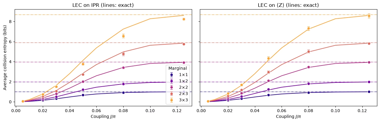
두 방법 모두 손상의 대부분을 제거합니다. 이전 플롯의 원시 추정값은 지나치게 무작위적이었지만 완화된 추정값은 정확한 곡선을 따라갑니다. 차이는 더 큰 주변 분포에서 나타납니다.
작은 주변 분포에서는 두 방법 모두 잘 작동합니다. 주변 분포에서는 에 대한 LEC가 확실히 더 가깝습니다.
IPR에 대한 LEC가 엔트로피를 너무 적게 주는 이유. 엔트로피가 너무 적다는 것은 IPR이 너무 크다는 뜻입니다. IPR에 대한 LEC는 IPR을 과도하게 부풀립니다. 이 방법은 노이즈가 모든 의 IPR 기여를 같은 인수로 감쇠시킨다고 가정합니다. 에서는 모든 가 에 가까우므로 모든 문자열이 동등하게 기여하고, 대부분의 문자열은 중간 가중치를 가집니다. 주변 분포의 511개 문자열 중 252개는 가중치가 4 또는 5이고 가중치가 1인 것은 아홉 개뿐입니다. 노이즈는 가중치가 높은 문자열일수록 더 많이 감쇠시키므로(판독 오류만으로도 가중치 인 문자열은 만큼 감쇠됩니다), 단일 인수 는 주로 중간 가중치 문자열의 감쇠에 의해 정해집니다. 가 커지면 가중치가 높은 가 가장 빨리 감소하고 IPR은 점점 더 가중치가 낮은 문자열이 담당하게 되는데, 이들은 노이즈로 인한 감쇠가 더 적습니다. 주로 더 많이 감쇠된 문자열에서 학습한 인수로 이들을 증폭하면 IPR이 과도하게 부풀려집니다. 주변 분포가 클수록 가중치의 범위가 넓으므로 이 효과도 커집니다. 문자열의 구성이 이미 바뀌었지만 IPR이 균일 값을 넘는 초과분이 여전히 중요한 중간 에서 가장 큽니다.
에 대한 LEC가 반대 방향으로 틀리는 이유. 이 방법은 각 문자열을 각자의 인수로 재조정하므로 가중치 간의 이동에 영향을 받지 않습니다. 각 문자열이 에서의 감쇠를 유지한다고만 가정합니다. 가 커지면 각 는 더 높은 가중치의 연산자로 퍼지고, 이들은 에서보다 더 많은 노이즈를 받으므로 인수가 약간 덜 보정하게 되어 엔트로피가 약간 너무 높게 나옵니다.
따라서 하드웨어에서 검증할 예측은 다음과 같습니다. 주변 분포가 클수록 에 대한 LEC가 더 유리해야 합니다. 하드웨어에서는 노이즈가 더 강하고 알려진 형태도 아닙니다.
4. 대규모 실행
하드웨어 실험은 네 주기의 격자, 즉 48개 레이어에 64큐비트와 1,344개의 CZ 게이트를 아홉 개의 결합에서 실행합니다. 시뮬레이션과 비교해 다섯 가지가 달라집니다.
-
노이즈를 학습해야 하며, 이는 CZ 레이어가 고정되어 있어야만 가능합니다.
-
**트위링(twirling)**은 각 레이어의 노이즈를 학습하고 증폭할 수 있는 Pauli 채널로 바꿉니다.
-
**동적 디커플링(DD)**은 유휴 큐비트를 보호합니다.
-
PEA를 위한 노이즈 증폭은 주요 데이터와 같은 작업에서 실행됩니다.
-
작은 에서의 MPS 시뮬레이션은 LEC 기반 오류 완화를 위한 고전 참조를 제공합니다.
백엔드가 필요한 셀은 RUN_ON_HARDWARE가 True일 때만 실행됩니다. MPS 시뮬레이션은 COMPUTE_MPS_REFERENCES를 True로 설정하면 다시 실행할 수 있습니다. 나머지 셀은 여기서 실행됩니다.
# hardware run parameters:
num_cols_hw = num_rows_hw = 8
num_qubits_hw = num_cols_hw * num_rows_hw
num_cycles_hw = 4
couplings_hw = (
    np.array([0.005, 0.01, 0.02, 0.03, 0.05, 0.07, 0.09, 0.11, 0.125]) * np.pi
)
calibration_hw = 0  # J0 = 0.005π
disorder_hw = sample_disorder(
    num_cols_hw, num_rows_hw, np.random.default_rng(7)
)

# if running PEA:
noise_factors = np.array([1.0, 1.5, 2.0])  # PEA noise-amplification factors
고정된 CZ 레이어
def compile_by_sublayer(
    num_cols,
    num_rows,
    coupling,
    num_cycles,
    disorder,
    pass_manager,
    layout=None,
    num_physical_qubits=None,
):
    # Compile each sublayer once and repeat it with barriers, so the CZ layers are the
    # same in every cycle and at every coupling. The registers are named explicitly
    # because register names enter Samplomatic's box hashes. Bits land in lattice order.
    num_qubits = num_cols * num_rows
    if layout is None:
        layout, num_physical_qubits = list(range(num_qubits)), num_qubits
    blocks = []
    for sublayer in disorder:
        block = QuantumCircuit(num_qubits)
        for (i, j), (h_i, h_j) in sublayer:
            heisenberg_gate(block, coupling, i, j, h_i, h_j)
        blocks.append(pass_manager.run(block))
    circuit = QuantumCircuit(
        QuantumRegister(num_physical_qubits, "q"),
        ClassicalRegister(num_qubits, "meas"),
    )
    neel_state(circuit, num_cols, num_rows, layout)
    for _ in range(num_cycles):
        for block in blocks:
            circuit.compose(block, inplace=True)
            circuit.barrier(layout)
    circuit.measure(layout, range(num_qubits))
    return circuit
노이즈 학습을 위한 박스
그런 다음 Samplomatic 박싱 패스 매니저가 각 회로를 CZ 레이어마다 하나, 측정에 하나씩의 박스로 묶습니다. 각 박스는 필요한 노이즈 모델에 대한 참조를 가지므로 모든 결합이 같은 박스를 공유하는지 확인할 수 있습니다. 다음 셀은 하드웨어 실행의 회로에 대해 이를 수행하고, 백엔드 없이 CZ 게이트로 컴파일한 뒤 노이즈 학습이 특성화할 박스를 출력합니다.
from samplomatic import build
from samplomatic.transpiler import generate_boxing_pass_manager
from samplomatic.utils import find_unique_box_instructions

boxing_pass_manager = generate_boxing_pass_manager(
    enable_gates=True,  # twirl the CZ layers
    enable_measures=True,  # twirl the measurements
    inject_noise_targets="gates",  # PEA amplifies the noise of the CZ layers only
    inject_noise_strategy="uniform_modification",
)

def noise_refs(boxed_circuit):
    return sorted(
        annotation.ref
        for box in find_unique_box_instructions(boxed_circuit.data)
        for annotation in box.operation.annotations
        if hasattr(annotation, "ref")
    )

# The 8x8 hardware circuits, compiled to CZ gates on the lattice qubits (no backend needed)
compiled_8x8 = [
    compile_by_sublayer(
        num_cols_hw, num_rows_hw, c, num_cycles_hw, disorder_hw, pass_manager
    )
    for c in couplings_hw
]
boxed_8x8 = [boxing_pass_manager.run(circuit) for circuit in compiled_8x8]
assert all(
    noise_refs(b) == noise_refs(boxed_8x8[0]) for b in boxed_8x8
), "layers differ between couplings"
num_cz, depth = two_qubit_stats(compiled_8x8[0])
print(
    f"{num_qubits_hw} qubits: {num_cz} CZ gates in {depth} layers, for every coupling"
)
for box in find_unique_box_instructions(boxed_8x8[0].data):
    ops = box.operation.blocks[0].count_ops()
    print(
        f"{box.operation.num_qubits}-qubit box: {ops.get('cz', 0)} CZ, {ops.get('measure', 0)} measurements"
    )
print(
    f"All {len(boxed_8x8)} couplings share these {len(find_unique_box_instructions(boxed_8x8[0].data))} boxes"
)
64 qubits: 1344 CZ gates in 48 layers, for every coupling
64-qubit box: 32 CZ, 0 measurements
64-qubit box: 24 CZ, 0 measurements
64-qubit box: 32 CZ, 0 measurements
64-qubit box: 24 CZ, 0 measurements
64-qubit box: 0 CZ, 64 measurements
All 9 couplings share these 5 boxes
회로 트위링
모든 무작위화에서 Samplomatic은 각 박스 앞에 무작위 Pauli 게이트를, 뒤에 이를 보상하는 게이트를 넣고 이웃한 단일 큐비트 게이트에 병합합니다. 무작위화에 대해 평균하면 각 레이어의 노이즈는 Pauli 채널이 되며, NoiseLearnerV3가 이를 희소 Pauli-Lindblad 모델로 학습하고 PEA 단계가 증폭할 수 있습니다. 측정 트위링은 판독 전에 비트를 무작위로 뒤집습니다. 뒤집힌 비트는 소프트웨어에서 되돌리며, 이로써 판독 노이즈가 대칭이 되고 판독 보정(TREX)의 기초가 됩니다.
하드웨어 워크플로
큐비트를 선택하고 회로를 컴파일한 다음 노이즈를 학습하고 스윕을 실행합니다. 이 셀들은 여기서는 꺼져 있습니다.
큐비트 선택. Nighthawk의 정사각 격자는 SWAP 게이트 없이 격자를 담을 수 있습니다. 이 셀은 격자의 모든 사각형을 보고된 CZ 및 판독 오류로 점수화하여 가장 좋은 것을 선택합니다.
def square_layouts(backend, side):
    # Every side x side rectangle of the square qubit grid that supports all bonds
    target = backend.target

    def has_cz(a, b):
        return (a, b) in target["cz"] or (b, a) in target["cz"]

    stride = next(
        s
        for s in (10, 12)
        if all(has_cz(q, q + s) for q in range(backend.num_qubits - s))
    )
    layouts = []
    for y0 in range(backend.num_qubits // stride - side + 1):
        for x0 in range(stride - side + 1):
            layout = [
                stride * (y0 + y) + x0 + x
                for y in range(side)
                for x in range(side)
            ]
            bonds = [
                bond
                for layer in brickwork_layers(side, side)
                for bond in layer
            ]
            if all(has_cz(layout[i], layout[j]) for i, j in bonds):
                layouts.append(((x0, y0), layout))
    return layouts

def layout_score(backend, layout, side, uses_per_bond):
    # Minus the summed log-fidelity of the bonds (each used uses_per_bond times) and readouts
    properties, target = backend.properties(), backend.target
    cz_errors = []
    for i, j in (
        bond for layer in brickwork_layers(side, side) for bond in layer
    ):
        pair = (
            (layout[i], layout[j])
            if (layout[i], layout[j]) in target["cz"]
            else (layout[j], layout[i])
        )
        cz_errors.append(properties.gate_error("cz", pair))
    readout_errors = [properties.readout_error(q) for q in layout]
    if max(cz_errors) >= 0.5 or max(readout_errors) >= 0.25:
        return np.inf  # an unusable qubit or bond
    return float(
        -uses_per_bond * np.log1p(-np.array(cz_errors)).sum()
        - np.log1p(-np.array(readout_errors)).sum()
    )

if RUN_ON_HARDWARE:
    from qiskit_ibm_runtime import QiskitRuntimeService

    def holds_lattice(backend):
        try:
            return bool(square_layouts(backend, num_cols_hw))
        except (KeyError, StopIteration):
            return False

    service = QiskitRuntimeService()
    candidates = [
        b
        for b in service.backends(operational=True, simulator=False)
        if holds_lattice(b)
    ]
    backend = min(candidates, key=lambda b: b.status().pending_jobs)
    score, origin, initial_layout = min(
        (
            layout_score(backend, layout, num_cols_hw, 3 * num_cycles_hw),
            origin,
            layout,
        )
        for origin, layout in square_layouts(backend, num_cols_hw)
    )
    print(f"{backend.name}: origin {origin}, score {score:.2f}")
컴파일. 선택한 큐비트에서 위와 같은 단계를 수행한 뒤 build를 실행합니다. 이는 박스로 묶인 각 회로를 템플릿 회로와 samplex, 즉 트위링 게이트와 주입된 노이즈를 뽑기 위한 레시피로 바꿉니다. DD는 템플릿에 추가됩니다.
if RUN_ON_HARDWARE:
    from qiskit_ibm_runtime.executor.dynamical_decoupling import (
        generate_dd_pass_manager,
    )
    from qiskit_ibm_runtime.options import DynamicalDecouplingOptions

    # PEA structure functions:
    target_pass_manager = generate_preset_pass_manager(
        target=backend.target,
        optimization_level=3,
        initial_layout=initial_layout,
        routing_method="none",
        seed_transpiler=7,
    )
    boxed_hw = [
        boxing_pass_manager.run(
            compile_by_sublayer(
                num_cols_hw,
                num_rows_hw,
                coupling,
                num_cycles_hw,
                disorder_hw,
                target_pass_manager,
                layout=initial_layout,
                num_physical_qubits=backend.num_qubits,
            )
        )
        for coupling in couplings_hw
    ]
    assert all(noise_refs(b) == noise_refs(boxed_hw[0]) for b in boxed_hw)
    unique_boxes_hw = find_unique_box_instructions(boxed_hw[0].data)

    # DD pass:
    dd_pass_manager = generate_dd_pass_manager(
        backend,
        DynamicalDecouplingOptions(
            enable=True,
            sequence_type="XY4",
            scheduling_method="alap",
            extra_slack_distribution="middle",
            skip_reset_qubits=False,
        ),
    )
    templates = []
    for circuit in boxed_hw:
        template, samplex = build(circuit)
        templates.append((dd_pass_manager.run(template), samplex))
노이즈 학습 및 스윕 실행. NoiseLearnerV3 작업 하나가 다섯 개의 박스를 모두 학습합니다. 네 개의 CZ 레이어 각각에 대한 Pauli-Lindblad 모델과 측정 박스의 판독 노이즈입니다. 그런 다음 QuantumProgram 하나에 아홉 개의 결합이 모두 담깁니다. 각 항목은 템플릿, samplex, 학습된 노이즈 모델, 세 가지 노이즈 스케일을 받습니다. 스케일 0은 두 LEC 방법을 위한 증폭되지 않은 데이터입니다. 스케일 0.5와 1은 PEA를 위해 학습된 노이즈의 50%와 100%를 추가하며, PEA는 노이즈가 0인 지점으로 외삽합니다. 이는 QPU 시간을 약 40초 사용합니다.
if RUN_ON_HARDWARE:
    from qiskit_ibm_runtime import Executor, NoiseLearnerV3, QuantumProgram

    # Learn the noise of the five boxes
    learner = NoiseLearnerV3(backend)
    learner.options.num_randomizations = 32
    learner.options.shots_per_randomization = 128
    # Up to 24 layer pairs, the depth of the 48-layer circuits
    learner.options.layer_pair_depths = [0, 1, 2, 4, 16, 24]
    learner_job = learner.run(unique_boxes_hw)
    print("Noise learning job:", learner_job.job_id())

    # Run the sweep, with the learned noise amplified by each of the noise factors
    noise_maps = learner_job.result().to_dict(
        instructions=unique_boxes_hw, require_refs=False
    )
    program = QuantumProgram(shots=200)
    for template, samplex in templates:
        program.append_samplex_item(
            template,
            samplex=samplex,
            samplex_arguments={
                "pauli_lindblad_maps": noise_maps,
                **{
                    f"noise_scales.{ref}": (noise_factors - 1).reshape(-1, 1)
                    for ref in noise_maps
                },
            },
            shape=(len(noise_factors), 200),  # noise scales x randomizations
        )
    executor_job = Executor(backend).run(program)
    print("Executor job:", executor_job.job_id())
    # Section 5 converts the results of these two jobs and saves them
5. 하드웨어 데이터
이 섹션에서는 앞선 방법들이 Nighthawk 프로세서의 실제 하드웨어 데이터에서 어떻게 작동하는지 살펴봅니다.
실행 불러오기
RUN_ON_HARDWARE가 True로 설정되어 있으면 다음 셀은 4번 섹션의 두 작업 결과를 변환하여 저장된 실행과 같은 형식으로 data/hardware_run_new.npz에 저장하므로, 새 실행을 나중에 다시 분석할 수 있습니다. 그렇지 않으면 data/hardware_run.npz에서 저장된 실행을 불러옵니다. 비트는 공간을 절약하기 위해 큐비트 축을 따라 묶여 있습니다.
작업이 실행되는 동안 커널이 재시작되더라도 작업을 다시 제출하지 마세요. 4번 섹션의 마지막 호출 이전의 셀들을 다시 실행하고, 같은 큐비트가 선택되는지 확인한 다음, 4번 섹션에서 출력된 작업 ID로 learner_job과 executor_job을 service.job(job_id)로 설정하세요.
if RUN_ON_HARDWARE:

    def unflip(item_result):
        # Undo the measurement twirling of an Executor item: flip back the bits that were flipped
        return item_result["meas"] ^ item_result["measurement_flips.meas"]

    learner_result = learner_job.result()
    raw_bits = [unflip(item) for item in executor_job.result()]

    # The learned readout map indexes the measured qubits in ascending physical order;
    # relabel it to lattice order
    measurement_box_index = next(
        k
        for k, box in enumerate(unique_boxes_hw)
        if "measure" in box.operation.blocks[0].count_ops()
    )
    measurement_box = next(
        inst
        for inst in boxed_hw[0].data
        if inst.operation.name == "box"
        and "measure" in inst.operation.blocks[0].count_ops()
    )
    measured = sorted(
        boxed_hw[0].find_bit(q).index for q in measurement_box.qubits
    )
    lattice_index = {physical: q for q, physical in enumerate(initial_layout)}
    readout_map = (
        learner_result[measurement_box_index]
        .to_pauli_lindblad_map()
        .apply_layout([lattice_index[p] for p in measured], num_qubits_hw)
    )

    # Save the run in the same format as the saved run, so it can be analyzed again later
    terms = readout_map.to_sparse_list()
    np.savez_compressed(
        "data/hardware_run_new.npz",
        bits=np.packbits(np.stack(raw_bits), axis=-1, bitorder="little"),
        labels=np.array([label for label, _, _ in terms]),
        indices=np.concatenate(
            [np.asarray(support) for _, support, _ in terms]
        ),
        rates=np.array([rate for _, _, rate in terms]),
        physical_qubits=np.array(initial_layout),
        couplings_over_pi=couplings_hw / np.pi,
        noise_factors=noise_factors,
    )
else:
    saved = np.load(
        "data/hardware_run.npz"
    )  # or data/hardware_run_new.npz, for a new run
    raw_bits = list(
        np.unpackbits(
            saved["bits"], axis=-1, count=num_qubits_hw, bitorder="little"
        ).astype(bool)
    )
    labels = [str(label) for label in saved["labels"]]
    indices = np.split(
        saved["indices"], np.cumsum([len(label) for label in labels])[:-1]
    )
    readout_map = PauliLindbladMap.from_sparse_list(
        list(zip(labels, indices, saved["rates"])), num_qubits_hw
    )

print(f"{len(raw_bits)} couplings, bits per coupling: {raw_bits[0].shape}")
print(
    f"Readout noise: {readout_map.num_terms} terms on {readout_map.num_qubits} qubits"
)
9 couplings, bits per coupling: (3, 200, 200, 64)
Readout noise: 64 terms on 64 qubits
고전 참조
두 LEC 방법 모두 에서의 이상적인 주변 분포가 필요하며, 이를 테스트하려면 보류된 결합 와 에서의 이상적인 값이 필요합니다. 이 값들은 논문에서와 같이 격자 위 각 주변 분포 형태의 모든 배치와 에서 겹치지 않는 모든 블록에 대해 저장된 행렬곱 상태(MPS) 시뮬레이션에서 나옵니다. 에서는 본드 차원 에서 수렴합니다. 와 에서는 을 사용하며, 에서는 주변 분포에 대해 와 비교해 여전히 최대 약 13%까지 달라지므로 그곳의 값은 근사치로 취급하세요. 다음 셀은 COMPUTE_MPS_REFERENCES가 True이면 이를 계산하며 약 18분이 걸리고, 그렇지 않으면 결합 인덱스, 본드 차원, 주변 분포를 키로 하는 저장된 결과를 불러옵니다.
# Every placement of every shape on the 8x8 lattice
positions = {
    label: all_positions(shape, num_cols_hw, num_rows_hw)
    for label, shape in patch_shapes.items()
}
reference_settings = [
    (calibration_hw, 32),
    (calibration_hw, 64),
    (1, 128),
    (2, 64),
    (2, 128),
]  # (coupling, χ)

if COMPUTE_MPS_REFERENCES:

    def mps_patch_probabilities(coupling, patches, bond_dimension):
        # Distributions of the given marginals after the 8x8 circuit, from an MPS simulation
        simulator = AerSimulator(
            method="matrix_product_state",
            matrix_product_state_max_bond_dimension=bond_dimension,
            matrix_product_state_truncation_threshold=1e-12,
        )
        circuit = heisenberg_floquet_circuit(
            num_cols_hw,
            num_rows_hw,
            coupling,
            num_cycles_hw,
            disorder_hw,
            measure=False,
        )
        circuit = generate_preset_pass_manager(
            optimization_level=1, basis_gates=["cx", "u"], seed_transpiler=7
        ).run(circuit)
        for label, qubits in patches.items():
            circuit.save_probabilities(qubits, label=label)
        data = simulator.run(circuit, shots=1).result().data(0)
        return {label: np.asarray(data[label]) for label in patches}

    placements = {
        f"{label} {k}": qubits
        for label, patch_list in positions.items()
        for k, qubits in enumerate(patch_list)
    }
    tiles = {
        f"site {q}": [q] for q in range(num_qubits_hw)
    } | {  # for the lattice map at J0
        f"block {x},{y}": patch_qubits((2 * x, 2 * y), (2, 2), num_cols_hw)
        for y in range(num_rows_hw // 2)
        for x in range(num_cols_hw // 2)
    }
    computed = {}
    for index, chi in reference_settings:
        targets = (
            placements | tiles
            if (index, chi) == (calibration_hw, 64)
            else placements
        )
        for key, p in mps_patch_probabilities(
            couplings_hw[index], targets, chi
        ).items():
            computed[f"{index}/{chi}/{key}"] = p
    np.savez_compressed("data/mps_references_all.npz", **computed)
    saved = computed
else:
    saved = np.load("data/mps_references_all.npz")

references = {}  # (coupling index, bond dimension) -> {marginal key: distribution}
for name in saved:
    index, chi, key = name.split("/", 2)
    references.setdefault((int(index), int(chi)), {})[key] = saved[name]
데이터 품질: 결함 있는 커플러/큐비트
먼저 기댓값이 Néel 체커보드에 가까워야 하는 가장 낮은 결합 을 살펴보세요.
# <Z> of every site at J0: the MPS reference, and the hardware data at noise factor 1
z_reference = np.array(
    [
        parities_from_probabilities(
            references[(calibration_hw, 64)][f"site {q}"]
        )[0]
        for q in range(num_qubits_hw)
    ]
)
z_measured = 1 - 2 * raw_bits[calibration_hw][0].mean(axis=(0, 1))
fig, axes = plt.subplots(1, 2, figsize=(11, 4.6), layout="constrained")
fig.get_layout_engine().set(wspace=0.12)  # white space between the two panels
edges = np.arange(num_cols_hw + 1) - 0.5
for ax, values, title in zip(
    axes, (z_reference, z_measured), ("MPS reference", "Hardware")
):
    mesh = ax.pcolormesh(
        edges,
        edges,
        values.reshape(num_rows_hw, num_cols_hw),
        cmap="RdBu_r",
        vmin=-1,
        vmax=1,
        edgecolors="white",
    )
    ax.set_aspect("equal")
    ax.invert_yaxis()
    ax.set_xticks([])
    ax.set_yticks([])
    ax.set_title(
        f"{title}, $J_0 = {couplings_hw[calibration_hw] / np.pi:g}\\pi$"
    )
fig.colorbar(
    mesh, ax=axes, shrink=0.8, label=r"$\langle Z \rangle$ of each site"
)
plt.show()

질문. 하드웨어 맵을 보면 무엇이 눈에 띄나요?
정답
에서의 상태가 Néel 상태에 가까운데도 신호를 거의 모두 잃은 옅은 사이트들입니다. LEC는 에서 남아 있는 신호로 나누기 때문에 이것이 중요합니다. 신호가 거의 없는 큐비트는 매우 크고 노이즈가 많은 보정 인수를 주며, 이런 큐비트 몇 개가 그것을 포함하는 모든 주변 분포를 좌우할 수 있습니다.
데이터만 사용하는 규칙: 에서 단일 큐비트 IPR이 완전 혼합 큐비트의 값인 에서 이내이면 그 큐비트는 결함이 있는 것입니다. 큐비트 하나의 IPR은 이므로 이 규칙은 인 큐비트를 표시합니다. 표시된 사이트를 포함하는 주변 분포는 아래에서 제외됩니다.
site_iprs = np.array(
    [
        ipr_from_shots(raw_bits[calibration_hw][0][:, :, [q]])
        for q in range(num_qubits_hw)
    ]
)
# |IPR - 1/2| < 0.25**2 / 2 is the same as |<Z>| < 0.25
flagged = {
    q for q in range(num_qubits_hw) if abs(site_iprs[q] - 0.5) < 0.25**2 / 2
}
print(
    f"Median single-qubit IPR at J0: {np.median(site_iprs):.2f}; flagged lattice sites {sorted(flagged)}"
)
Median single-qubit IPR at J0: 0.77; flagged lattice sites [19, 24, 25, 27, 32]
평균을 낼 주변 분포 선택
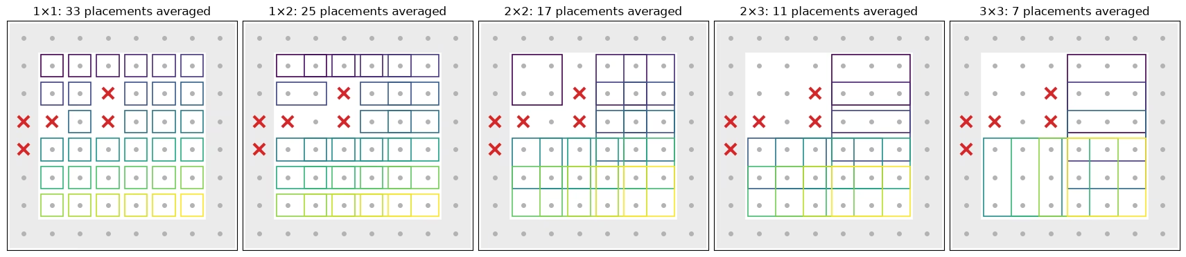
다음 셀은 아래 평균에 포함되는 각 모양의 배치를 보여 줍니다. 격자의 내부(bulk)에 있으면서 표시된 사이트(빨간 십자)가 없는 모든 배치가 포함됩니다. 가장자리에 닿는 배치(음영 처리)는 제외됩니다. 가장자리 큐비트는 결합이 더 적어서 스크램블링이 더 느립니다. 가장자리 큐비트만 따로 평균을 내면, 모든 모양과 방법에서 내부 배치보다 가 한 단계 전체만큼 더 커진 뒤에 교차합니다. 평균에 사용된 각 배치에는 배치별로 색을 입힌 고유한 상자가 있습니다.
def touches_edge(qubits):
    # Whether a placement includes a site on the edge of the lattice
    return any(
        q % num_cols_hw in (0, num_cols_hw - 1)
        or q // num_cols_hw in (0, num_rows_hw - 1)
        for q in qubits
    )

# The placements of each shape that enter the averages: in the bulk, and without a flagged site
kept_placements = {
    label: [
        k
        for k, qubits in enumerate(patch_list)
        if not touches_edge(qubits) and not set(qubits) & flagged
    ]
    for label, patch_list in positions.items()
}
placement_cmap = plt.get_cmap("viridis")
fig, axes = plt.subplots(
    1, len(positions), figsize=(17, 4.4), layout="constrained"
)
for ax, (label, patch_list) in zip(axes, positions.items()):
    width, height = patch_shapes[label]
    for q in range(num_qubits_hw):
        x, y = q % num_cols_hw, q // num_cols_hw
        if touches_edge([q]):  # shade the edge of the lattice
            ax.add_patch(
                plt.Rectangle(
                    (x - 0.5, y - 0.5), 1, 1, color="0.92", zorder=0
                )
            )
        ax.plot(x, y, "o", color="0.7", ms=4, zorder=1)
    kept = kept_placements[label]
    for i, k in enumerate(kept):
        qubits = patch_list[k]
        x0, y0 = (
            qubits[0] % num_cols_hw,
            qubits[0] // num_cols_hw,
        )  # top-left site of the placement
        ax.add_patch(
            plt.Rectangle(
                (x0 - 0.4, y0 - 0.4),
                width - 0.2,
                height - 0.2,
                fill=False,
                lw=1.2,
                ec=placement_cmap(i / max(len(kept) - 1, 1)),
                zorder=2,
            )
        )
    for q in flagged:
        ax.plot(
            q % num_cols_hw,
            q // num_cols_hw,
            "x",
            color="#d62728",
            ms=11,
            mew=3,
            zorder=3,
        )
    ax.set_xlim(-0.6, num_cols_hw - 0.4)
    ax.set_ylim(num_rows_hw - 0.4, -0.6)
    ax.set_aspect("equal")
    ax.set_xticks([])
    ax.set_yticks([])
    ax.set_title(f"{label}: {len(kept)} placements averaged")
plt.show()
PEA
세 번째 방법은 고전적인 기준이 필요하지 않습니다. 각 패리티에 대해 노이즈 계수 1, 1.5, 2에서의 값을 가져와 학습된 판독 감쇠(TREX)를 나누어 제거하고, 노이즈 계수에 대한 지수 함수를 피팅한 다음 노이즈가 0인 지점으로 외삽합니다. 부호가 바뀌거나 거의 0에 가까운 패리티에는 직선 피팅을 사용합니다. 분산을 빼려면 분산의 신뢰할 만한 추정치가 필요한데, 원시 패리티와 재조정된 패리티에서는 이것이 쉽지만 클리핑과 대체 규칙이 있는 비선형 피팅의 출력에서는 쉽지 않습니다. 그래서 PEA는 제곱의 편향을 제거하는 또 다른 표준 방법을 사용합니다. 무작위화의 절반씩을 따로 외삽한 뒤, 두 독립 추정치를 곱합니다.
def readout_fidelity(support):
    # Damping of <Z_S> by the learned readout noise
    pauli = QubitSparsePauli.from_sparse_label(
        ("Z" * len(support), list(support)), num_qubits_hw
    )
    return readout_map.pauli_fidelity(pauli)

def extrapolate_to_zero(values):
    # Fit a * exp(b * factor) to each column of values (noise factors first), or a line
    # where the values change sign or come within 1e-3 of zero
    result = np.polynomial.polynomial.polyfit(noise_factors, values, 1)[0]
    sign = np.sign(values[0])
    usable = np.all(np.sign(values) == sign, axis=0) & (
        np.abs(values).min(axis=0) > 1e-3
    )
    if usable.any():
        log_fit = np.polynomial.polynomial.polyfit(
            noise_factors, np.log(np.abs(values[:, usable])), 1
        )
        result[usable] = sign[usable] * np.exp(log_fit[0])
    return result

def pea_ipr(parities, fidelities, num_patch):
    # parities has shape (noise factors, randomizations, supports). Extrapolate the two
    # halves of the randomizations separately; their errors are independent, so the
    # product of the two estimates of each parity has no shot-noise bias
    def zero_noise(p):
        # A parity cannot exceed 1 in magnitude, so cap the extrapolated values there
        return np.clip(
            extrapolate_to_zero(p.mean(axis=1) / fidelities), -1, 1
        )

    half = parities.shape[1] // 2
    first, second = (
        zero_noise(parities[:, :half]),
        zero_noise(parities[:, half:]),
    )
    return float((1 + np.dot(first, second)) / 2**num_patch)
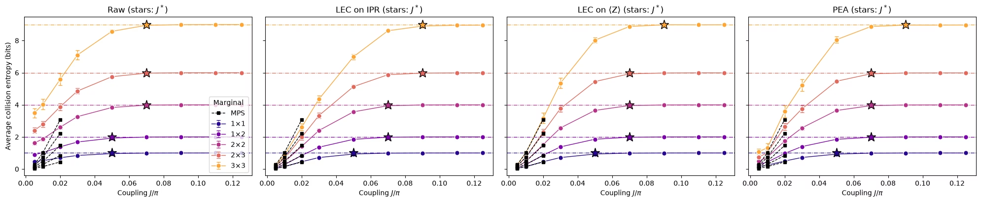
네 가지 추정치 전체와 교차점
다음 함수는 모든 결합 세기에서 한 주변 분포 위치의 IPR에 대해 원시, LEC-on-IPR, LEC-on-, PEA 추정치를 계산합니다. 또한 무작위화를 부트스트래핑하여 각 추정치의 샷 노이즈도 추정합니다. 이 셀은 평균에 들어가는 모든 배치에 대해 함수를 실행하며, 약 1분 30초가 걸립니다.
def estimate_iprs(qubits, key):
    # Raw, LEC-on-IPR, LEC-on-<Z>, and PEA IPRs of one marginal position at every coupling,
    # with the shot noise of each from a bootstrap over the randomizations
    n = len(qubits)
    supports = parity_supports(qubits)
    # Parities with shape (noise factors, randomizations, supports), per coupling
    parities = [
        np.stack([parity_expectation_values(b, supports) for b in bits])
        for bits in raw_bits
    ]
    patch_bits = [
        bits[0][:, :, qubits] for bits in raw_bits
    ]  # noise factor 1
    values, errors = lec_estimates(
        patch_bits,
        [p[0] for p in parities],
        references[(calibration_hw, 64)][key],
        calibration_hw,
        n,
    )
    fidelities = np.array([readout_fidelity(s) for s in supports])

    def pea_statistic(p):
        return pea_ipr(p, fidelities, n)

    values["raw"] = [ipr_from_shots(b) for b in patch_bits]
    errors["raw"] = [bootstrap_error(ipr_from_shots, b) for b in patch_bits]
    values["PEA"] = [pea_statistic(p) for p in parities]
    errors["PEA"] = [
        bootstrap_error(pea_statistic, p, axis=1) for p in parities
    ]  # randomizations are axis 1
    return {m: np.array(v) for m, v in values.items()}, {
        m: np.array(e) for m, e in errors.items()
    }

methods = ["LEC on IPR", "LEC on ⟨Z⟩", "PEA"]
method_colors = {
    "LEC on IPR": "#2a78d6",
    "LEC on ⟨Z⟩": "#1baf7a",
    "PEA": "#eb6834",
}
iprs, ipr_errors = {}, {}
for label, patch_list in positions.items():
    for k in kept_placements[label]:
        iprs[label, k], ipr_errors[label, k] = estimate_iprs(
            patch_list[k], f"{label} {k}"
        )
print(f"{len(iprs)} clean marginal positions")
93 clean marginal positions
def crossover_coupling(couplings, entropies, haar, tolerance=0.1):
    # Smallest coupling whose entropy is within tolerance of the random-state value
    for coupling, entropy in zip(couplings, entropies):
        if entropy >= haar - tolerance:
            return coupling
    return None

def reference_ipr(index, chi, key):
    # IPR of the MPS distribution of a marginal
    return float((references[(index, chi)][key] ** 2).sum())

mps_settings = [
    (calibration_hw, 64),
    (1, 128),
    (2, 128),
]  # (coupling index, bond dimension)
panels = ["raw", *methods]

# Average IPR of every shape over its clean placements, then the entropy and the crossover
hw_entropies = {
    method: {} for method in panels
}  # per method and shape: average entropy and its error
crossovers = {method: {} for method in panels}
mps_entropies = {}  # per shape: MPS entropy, averaged over the same placements, at mps_settings
for label, patch_list in positions.items():
    haar = haar_entropy(len(patch_list[0]), num_qubits_hw)
    keys = [(shape, k) for (shape, k) in iprs if shape == label]
    mps_entropies[label] = [
        collision_entropy(
            np.mean([reference_ipr(j, chi, f"{label} {k}") for _, k in keys])
        )
        for j, chi in mps_settings
    ]
    for method in panels:
        ipr, ipr_error = average_ipr(
            [iprs[key][method] for key in keys],
            [ipr_errors[key][method] for key in keys],
        )
        entropy = collision_entropy(ipr)
        hw_entropies[method][label] = (entropy, ipr_error / (ipr * np.log(2)))
        crossovers[method][label] = crossover_coupling(
            couplings_hw, entropy, haar
        )
fig, axes = plt.subplots(
    1, len(panels), figsize=(5 * len(panels), 4.2), sharey=True
)
for (label, patch_list), color in zip(positions.items(), colors):
    haar = haar_entropy(len(patch_list[0]), num_qubits_hw)
    for ax, method in zip(axes, panels):
        entropy, error = hw_entropies[method][label]
        ax.errorbar(
            couplings_hw / np.pi,
            entropy,
            yerr=error,
            fmt="o-",
            color=color,
            mec="white",
            ms=7,
            lw=1,
            capsize=3,
            label=label,
        )
        ax.plot(
            couplings_hw[[j for j, _ in mps_settings]] / np.pi,
            mps_entropies[label],
            "s--",
            color="black",
            ms=4,
            lw=1,
            label="MPS" if label == "3×3" else None,
            zorder=4,
        )
        ax.axhline(haar, color=color, ls="dashdot", lw=0.9)
        if crossovers[method][label]:
            ax.plot(
                crossovers[method][label] / np.pi,
                haar,
                "*",
                ms=14,
                color=color,
                mec="black",
                zorder=3,
            )
for ax, method in zip(axes, panels):
    ax.set_title(f"{'Raw' if method == 'raw' else method} (stars: $J^*$)")
    ax.set_xlabel("Coupling $J/\\pi$")
axes[0].set_ylabel("Average collision entropy (bits)")
axes[0].legend(title="Marginal", loc="lower right")
fig.tight_layout()
plt.show()
마무리
이 규모의 실험을 실행하는 데 필요했던 것은 다음과 같습니다.
-
구조가 에 의존하지 않는 회로: 한 번에 한 서브레이어씩 컴파일하므로 하나의 노이즈 모델로 전체 스윕을 처리할 수 있습니다.
-
비트열에서 작동하는 추정기: 주변 분포의 IPR에는 쌍 세기(pair counting)를 사용하고, 입력이 완화된 기댓값일 때는 각 제곱 패리티에서 분산을 뺀 Parseval 형식을 사용합니다.
-
저렴한 고전적 기준점: 작은 에서의 이상적인 상태로 노이즈를 보정하고, 따로 떼어 둔 결합 세기로 보정을 검증합니다. IPR 전체가 아니라 각 를 개별적으로 보정하는 것이 큰 주변 분포들이 서로 일치하게 만드는 요인입니다.
-
힘든 작업을 위한 IBM 도구: Samplomatic 박스와 트월링,
NoiseLearnerV3, 동적 디커플링, 그리고 PEA를 위한 노이즈 증폭이 포함된Executor작업 하나. -
데이터만 사용하는 데이터 품질 검사.
다음 단계. 오류 완화를 더 깊이 다루려면 확률적 오류 증폭 및 음영 라이트콘을 사용하는 PEC 튜토리얼을 참조하세요.